Credit Scoring with Zettapark and Python Machine Learning Libraries

Overview

In this step-by-step tutorial, you will use Zettapark for Python, along with your favorite data analysis and visualization Python libraries and the popular scikit-learn machine learning library, to solve an end-to-end machine learning use case.

Prerequisites

Lakehouse account
Client-side Zettapark environment with the Zettapark library installed.

What You Will Learn

Learn how to implement an end-to-end machine learning pipeline using Zettapark for Python.
Develop using Zettapark for Python APIs and vectorized functions.
Perform data exploration, visualization, and preparation using popular Python libraries (Pandas, seaborn).
Perform machine learning using the scikit-learn Python package.
Deploy and use machine learning models for scoring using Zettapark for Python.

Steps

Step 1: Run the credit scoring setup notebook. This downloads the dataset and creates the databases and tables required for this demo. Make sure to customize config.json.
Step 2: Now you can run the credit scoring tutorial.

You can get the source code (Jupyter Notebook ipynb files) and data files from the GitHub repository.

Credit Scoring Setup Notebook with Zettapark for Python

1. Lakehouse Trial Account

The prerequisite is having a Lakehouse account. If you do not have a Lakehouse account, contact us for a free trial.

After signing up for the trial, bookmark the Lakehouse account URL and save your credentials, which will be needed in this lab.

This release requires Zettapark 0.1.2 or later.

2. Python Libraries

The following libraries are required to run this demo. In this section, add any Python libraries that are missing from your environment.

# !pip install -q --upgrade clickzetta_zettapark_python

# !pip install scikit-plot

# !pip install pyarrow==6.0.0

# !pip install seaborn

# !pip install matplotlib

3. File Downloads

3.1 Dataset

! curl -o data/credit_files.csv https://raw.githubusercontent.com/yunqiqiliang/clickzetta_quickstart/refs/heads/main/Zettapark-credit-scoring/data/credit_files.csv

% Total % Received % Xferd Average Speed Time Time Time Current Dload Upload Total Spent Left Speed 100 292k 100 292k 0 0 66280 0 0:00:04 0:00:04 --:--:-- 69100

! curl -o data/credit_request.csv https://raw.githubusercontent.com/yunqiqiliang/clickzetta_quickstart/refs/heads/main/Zettapark-credit-scoring/data/credit_request.csv

% Total % Received % Xferd Average Speed Time Time Time Current Dload Upload Total Spent Left Speed 100 6068 100 6068 0 0 2297 0 0:00:02 0:00:02 --:--:-- 2297

3.2 config.json Credentials File

Edit the following file with your Lakehouse account credentials and save it. It will be used to connect to Lakehouse in the main notebook:

{ "username": "<username>", "password": "<password>", "service": "<service url>", "instance": "<instance id>", "workspace": "<workspace>", "schema": "<schema>", "vcluster": "<vcluster>", "sdk_job_timeout": 60, "hints": { "sdk.job.timeout": 60, "query_tag": "test_zettapark_credit_scoring" } }

! curl -o config/config_tobe_renamed.json https://raw.githubusercontent.com/yunqiqiliang/clickzetta_quickstart/refs/heads/main/Zettapark-credit-scoring/config/config.json

% Total % Received % Xferd Average Speed Time Time Time Current Dload Upload Total Spent Left Speed 100 321 100 321 0 0 138 0 0:00:02 0:00:02 --:--:-- 138

4. Database

In the section below, fill in the different parameters in the config.json file to connect to your Lakehouse environment.

import pandas as pd import json from clickzetta.zettapark.session import Session import clickzetta.zettapark.functions as F import warnings warnings.filterwarnings("ignore", category=FutureWarning) # Read connection parameters from config file with open('config/config.json', 'r') as config_file: config = json.load(config_file) schema = config['schema'] vcluster = config['vcluster'] print("Connecting to Lakehouse.....\n") # Create session session = Session.builder.configs(config).create() session.sql(f"CREATE SCHEMA IF NOT EXISTS {schema}").collect() session.sql(f"CREATE VCLUSTER IF NOT EXISTS {vcluster} VCLUSTER_SIZE=1 VCLUSTER_TYPE = GENERAL").collect() print(session.sql("SELECT current_instance_id(), current_workspace(),current_workspace_id(), current_schema(), current_user(),current_user_id(), current_vcluster()").collect()) print("\nConnected!...\n")

5. Tables

This demo includes 2 tables:

CREDIT_FILES: This table contains the credit standing on current files and whether the loan is being repaid or has actual issues in terms of credit repayment. This dataset will be used for historical analysis and to build a machine learning model for scoring new applications.
CREDIT_REQUESTS: This table contains new credit requests that the bank needs to approve based on the ML algorithm.

5.1 CREDIT_FILES Table

After running the following commands, log in to your Lakehouse environment and verify the table has been created. It should have 2.9K rows.

credit_files = pd.read_csv('data/credit_files.csv') credit_files.columns = credit_files.columns.str.lower() session.sql("drop table if exists CREDIT_FILES").collect() session.write_pandas(credit_files,"CREDIT_FILES",auto_create_table='True', quote_identifiers=False)

<clickzetta.zettapark.table.Table at 0x7fe58538e990>

credit_df = session.table("CREDIT_FILES") credit_df.schema

StructType([StructField('`credit_request_id`', LongType(), nullable=True), StructField('`credit_amount`', LongType(), nullable=True), StructField('`credit_duration`', LongType(), nullable=True), StructField('`purpose`', StringType(), nullable=True), StructField('`installment_commitment`', LongType(), nullable=True), StructField('`other_parties`', StringType(), nullable=True), StructField('`credit_standing`', StringType(), nullable=True), StructField('`credit_score`', LongType(), nullable=True), StructField('`checking_balance`', DoubleType(), nullable=True), StructField('`savings_balance`', DoubleType(), nullable=True), StructField('`existing_credits`', LongType(), nullable=True), StructField('`assets`', StringType(), nullable=True), StructField('`housing`', StringType(), nullable=True), StructField('`qualification`', StringType(), nullable=True), StructField('`job_history`', LongType(), nullable=True), StructField('`age`', LongType(), nullable=True), StructField('`sex`', StringType(), nullable=True), StructField('`marital_status`', StringType(), nullable=True), StructField('`num_dependents`', LongType(), nullable=True), StructField('`residence_since`', LongType(), nullable=True), StructField('`other_payment_plans`', StringType(), nullable=True)])

credit_df.toPandas().head()

credit_df.toPandas().info()

<class 'pandas.core.frame.DataFrame'> RangeIndex: 2940 entries, 0 to 2939 Data columns (total 21 columns): # Column Non-Null Count Dtype --- ------ -------------- ----- 0 credit_request_id 2940 non-null int64 1 credit_amount 2940 non-null int64 2 credit_duration 2940 non-null int64 3 purpose 2940 non-null object 4 installment_commitment 2940 non-null int64 5 other_parties 271 non-null object 6 credit_standing 2940 non-null object 7 credit_score 2940 non-null int64 8 checking_balance 2940 non-null float64 9 savings_balance 2940 non-null float64 10 existing_credits 2940 non-null int64 11 assets 2489 non-null object 12 housing 2940 non-null object 13 qualification 2940 non-null object 14 job_history 2940 non-null int64 15 age 2940 non-null int64 16 sex 2940 non-null object 17 marital_status 2940 non-null object 18 num_dependents 2940 non-null int64 19 residence_since 2940 non-null int64 20 other_payment_plans 2940 non-null object dtypes: float64(2), int64(10), object(9) memory usage: 482.5+ KB

5.2 CREDIT_REQUEST Table

After running the following commands, log in to your Lakehouse environment and verify the table has been created. It should have 60 rows.

credit_requests = pd.read_csv('data/credit_request.csv') credit_requests.columns = credit_requests.columns.str.lower() session.sql("drop table if exists CREDIT_REQUESTS").collect() session.write_pandas(credit_requests,"CREDIT_REQUESTS",auto_create_table='True', quote_identifiers=False)

<clickzetta.zettapark.table.Table at 0x7fe50b7556d0>

credit_req_df = session.table("CREDIT_REQUESTS") credit_req_df.schema

StructType([StructField('`credit_request_id`', LongType(), nullable=True), StructField('`credit_amount`', LongType(), nullable=True), StructField('`credit_duration`', LongType(), nullable=True), StructField('`purpose`', StringType(), nullable=True), StructField('`installment_commitment`', LongType(), nullable=True), StructField('`other_parties`', StringType(), nullable=True), StructField('`credit_score`', LongType(), nullable=True), StructField('`checking_balance`', DoubleType(), nullable=True), StructField('`savings_balance`', DoubleType(), nullable=True), StructField('`existing_credits`', LongType(), nullable=True), StructField('`assets`', StringType(), nullable=True), StructField('`housing`', StringType(), nullable=True), StructField('`qualification`', StringType(), nullable=True), StructField('`job_history`', LongType(), nullable=True), StructField('`age`', LongType(), nullable=True), StructField('`sex`', StringType(), nullable=True), StructField('`marital_status`', StringType(), nullable=True), StructField('`num_dependents`', LongType(), nullable=True), StructField('`residence_since`', LongType(), nullable=True), StructField('`other_payment_plans`', StringType(), nullable=True)])

credit_req_df.toPandas().head()

credit_req_df.toPandas().info()

<class 'pandas.core.frame.DataFrame'> RangeIndex: 60 entries, 0 to 59 Data columns (total 20 columns): # Column Non-Null Count Dtype --- ------ -------------- ----- 0 credit_request_id 60 non-null int64 1 credit_amount 60 non-null int64 2 credit_duration 60 non-null int64 3 purpose 60 non-null object 4 installment_commitment 60 non-null int64 5 other_parties 8 non-null object 6 credit_score 60 non-null int64 7 checking_balance 60 non-null float64 8 savings_balance 60 non-null float64 9 existing_credits 60 non-null int64 10 assets 49 non-null object 11 housing 60 non-null object 12 qualification 60 non-null object 13 job_history 60 non-null int64 14 age 60 non-null int64 15 sex 60 non-null object 16 marital_status 60 non-null object 17 num_dependents 60 non-null int64 18 residence_since 60 non-null int64 19 other_payment_plans 60 non-null object dtypes: float64(2), int64(10), object(8) memory usage: 9.5+ KB

Credit Scoring with Zettapark for Python

In this notebook, we will use the Zettapark Python API for a credit scoring demo.

In this scenario, Zettabank wants to leverage its existing credit files to analyze the current credit standing, i.e., whether loans are being repaid smoothly or if there are any delays/defaults.

Based on the current credit standing, Zettabank wants to build a machine learning credit scoring algorithm on the dataset to automatically assess whether a loan should be approved or denied.

Prerequisites

Please run the credit scoring demo setup notebook before running this demo.

1. Data Exploration

In this section, we will explore the dataset of existing credits.

1.1 Open a Lakehouse Session

import json import pandas as pd from clickzetta.zettapark import * from clickzetta.zettapark.functions import *

# Read connection parameters from config file with open('config/config.json', 'r') as config_file: config = json.load(config_file) schema = config['schema'] vcluster = config['vcluster'] print("Connecting to Lakehouse.....\n") # Create session session = Session.builder.configs(config).create() session.sql(f"CREATE SCHEMA IF NOT EXISTS {schema}").collect() session.sql(f"CREATE VCLUSTER IF NOT EXISTS {vcluster} VCLUSTER_SIZE=1 VCLUSTER_TYPE = GENERAL").collect() print(session.sql("SELECT current_instance_id(), current_workspace(),current_workspace_id(), current_schema(), current_user(),current_user_id(), current_vcluster()").collect()) print("\nConnected!...\n")

1.2 Explore Data in Lakehouse Tables

credit_df = session.table("CREDIT_FILES")

credit_df.describe().toPandas()

credit_df.toPandas().info()

credit_df.toPandas()

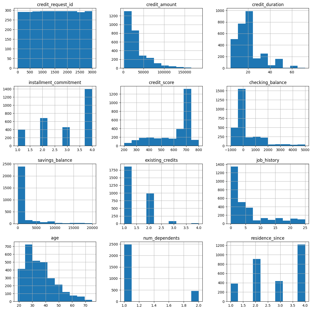
1.3 Visualize Numerical Features

From this visualization, we can observe some interesting characteristics:

Most credit requests are for smaller amounts (<50k)
Most credit durations are 20 months or shorter
Most applicants have high credit scores
Most applicants do not have large balances in their checking or savings accounts at Zettabank
Most applicants are under 40 years old

credit_df.toPandas().hist(figsize=(15,15))

array([[<Axes: title={'center': 'credit_request_id'}>, <Axes: title={'center': 'credit_amount'}>, <Axes: title={'center': 'credit_duration'}>], [<Axes: title={'center': 'installment_commitment'}>, <Axes: title={'center': 'credit_score'}>, <Axes: title={'center': 'checking_balance'}>], [<Axes: title={'center': 'savings_balance'}>, <Axes: title={'center': 'existing_credits'}>, <Axes: title={'center': 'job_history'}>], [<Axes: title={'center': 'age'}>, <Axes: title={'center': 'num_dependents'}>, <Axes: title={'center': 'residence_since'}>]], dtype=object)

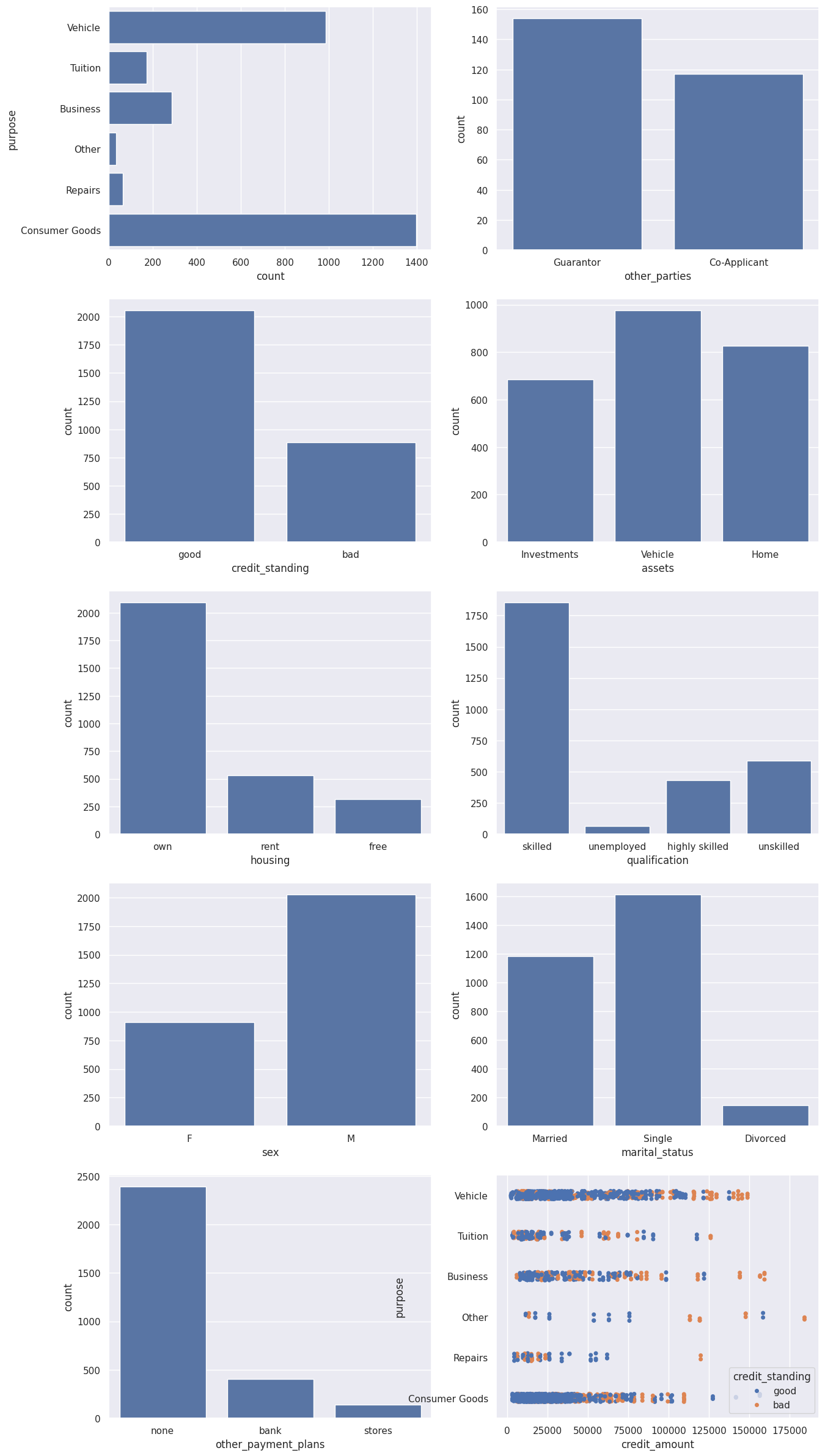
1.4 Visualize Categorical Features

From this visualization, we can observe some interesting characteristics:

The most popular credit requests are related to vehicle purchases or consumer goods
The vast majority of loans have neither a guarantor nor a co-applicant
Most credit standings in the files are good
Most applicants are male, foreign workers, skilled workers, and own their homes/apartments
Higher-amount loans (thresholds vary by loan category) have a higher likelihood of default

import matplotlib.pyplot as plt import seaborn as sns sns.set(style="darkgrid") fig, axs = plt.subplots(5, 2, figsize=(15, 30)) df = credit_df.toPandas() sns.countplot(data=df, y="purpose", ax=axs[0,0]) sns.countplot(data=df, x="other_parties", ax=axs[0,1]) sns.countplot(data=df, x="credit_standing", ax=axs[1,0]) sns.countplot(data=df, x="assets", ax=axs[1,1]) sns.countplot(data=df, x="housing", ax=axs[2,0]) sns.countplot(data=df, x="qualification", ax=axs[2,1]) sns.countplot(data=df, x="sex", ax=axs[3,0]) sns.countplot(data=df, x="marital_status", ax=axs[3,1]) sns.countplot(data=df, x="other_payment_plans", ax=axs[4,0]) sns.stripplot(y="purpose", x="credit_amount", data=df, hue='credit_standing', jitter=True, ax=axs[4,1]) plt.show()

1.5 Run Queries via Zettapark API

We can use Zettapark API to run queries to obtain various insights. For example, let's try to determine the loan ranges across different categories. We can check the Lakehouse query history to understand how Zettapark APIs are being pushed down as SQL.

df_loan_status = credit_df.select(col("PURPOSE"),col("CREDIT_AMOUNT"))\ .groupBy(col("PURPOSE"))\ .agg([min(col("CREDIT_AMOUNT")).as_("MIN_CREDIT_AMOUNT"), max(col("CREDIT_AMOUNT")).as_("MAX_CREDIT_AMOUNT"), median(col("CREDIT_AMOUNT")).as_("MED_CREDIT_AMOUNT"),avg(col("CREDIT_AMOUNT")).as_("AVG_CREDIT_AMOUNT")])\ .sort(col("PURPOSE")) df_loan_status.toPandas()

2. Data Transformation and Encoding

For this use case, to prepare the data into a format required for machine learning, we need to encode categorical values into numerical ones.

To achieve this, we can leverage Zettapark Python API for encoding.

2.1 Prepare Feature Matrix for Machine Learning

In this section, we will use the Zettapark Python API to prepare a feature matrix for a Random Forest classifier model.

from clickzetta.zettapark.functions import when feature_matrix = credit_df.select( when(col("purpose") == "Consumer Goods", 1) .when(col("purpose") == "Vehicle", 2) .when(col("purpose") == "Tuition", 3) .when(col("purpose") == "Business", 4) .when(col("purpose") == "Repairs", 5) .otherwise(0).alias("purpose_code"), when(col("qualification") == "unskilled", 1) .when(col("qualification") == "skilled", 2) .when(col("qualification") == "highly skilled", 3) .otherwise(0).alias("qualification_code"), when(col("other_parties") == "Guarantor", 1) .when(col("other_parties") == "Co-Applicant", 2) .otherwise(0).alias("other_parties_code"), when(col("other_payment_plans") == "bank", 1) .when(col("other_payment_plans") == "stores", 2) .otherwise(0).alias("other_payment_plans_code"), when(col("housing") == "rent", 1) .when(col("housing") == "own", 2) .otherwise(0).alias("housing_code"), when(col("assets") == "Vehicle", 1) .when(col("assets") == "Investments", 2) .when(col("assets") == "Home", 3) .otherwise(0).alias("assets_code"), when(col("sex") == "M", 1) .otherwise(0).alias("sex_code"), when(col("marital_status") == "Married", 1) .when(col("marital_status") == "Single", 2) .otherwise(0).alias("marital_status_code"), when(col("credit_standing") == "good", 1) .otherwise(0).alias("credit_standing_code"), col("checking_balance"), col("savings_balance"), col("age"), col("job_history"), col("credit_score"), col("credit_duration"), col("credit_amount"), col("residence_since"), col("installment_commitment"), col("num_dependents"), col("existing_credits") ) feature_matrix_pandas = feature_matrix.toPandas() print(feature_matrix_pandas)

purpose_code qualification_code other_parties_code \ 0 2 2 0 1 2 2 0 2 3 2 0 3 3 2 0 4 2 2 0 ... ... ... ... 2935 0 0 0 2936 2 0 0 2937 2 0 0 2938 2 2 0 2939 2 2 0 other_payment_plans_code housing_code assets_code sex_code \ 0 0 2 0 0 1 1 1 0 1 2 0 1 2 0 3 1 1 2 0 4 0 2 2 0 ... ... ... ... ... 2935 1 0 0 1 2936 1 0 0 1 2937 0 0 1 1 2938 0 2 1 1 2939 0 2 1 1 marital_status_code credit_standing_code checking_balance \ 0 1 1 -728.12 1 2 1 0.00 2 1 1 4696.00 3 1 1 -25.35 4 1 1 0.00 ... ... ... ... 2935 2 1 1505.00 2936 2 1 4486.00 2937 2 1 720.00 2938 2 1 752.00 2939 2 1 1564.00 savings_balance age job_history credit_score credit_duration \ 0 17.00 39 15 466 6 1 2443.00 35 1 202 6 2 143.00 23 1 736 15 3 0.00 23 3 732 12 4 510.00 30 1 507 18 ... ... ... ... ... ... 2935 0.00 40 0 726 48 2936 7361.86 66 0 343 12 2937 460.00 68 0 396 16 2938 1444.00 27 0 523 45 2939 1998.00 27 0 552 45 credit_amount residence_since installment_commitment num_dependents \ 0 8600 4 1 1 1 12040 1 4 1 2 3920 4 4 1 3 12000 4 4 1 4 10550 1 4 1 ... ... ... ... ... 2935 53810 4 3 1 2936 14800 4 2 1 2937 11750 3 2 1 2938 45760 4 3 1 2939 45760 4 3 1 existing_credits 0 2 1 1 2 1 3 1 4 2 ... ... 2935 1 2936 3 2937 3 2938 1 2939 1 [2940 rows x 20 columns]

Now that the feature matrix is defined, we convert it to a Pandas DataFrame.

df = feature_matrix.toPandas().astype(int)

df.info()

<class 'pandas.core.frame.DataFrame'> RangeIndex: 2940 entries, 0 to 2939 Data columns (total 20 columns): # Column Non-Null Count Dtype --- ------ -------------- ----- 0 purpose_code 2940 non-null int64 1 qualification_code 2940 non-null int64 2 other_parties_code 2940 non-null int64 3 other_payment_plans_code 2940 non-null int64 4 housing_code 2940 non-null int64 5 assets_code 2940 non-null int64 6 sex_code 2940 non-null int64 7 marital_status_code 2940 non-null int64 8 credit_standing_code 2940 non-null int64 9 checking_balance 2940 non-null int64 10 savings_balance 2940 non-null int64 11 age 2940 non-null int64 12 job_history 2940 non-null int64 13 credit_score 2940 non-null int64 14 credit_duration 2940 non-null int64 15 credit_amount 2940 non-null int64 16 residence_since 2940 non-null int64 17 installment_commitment 2940 non-null int64 18 num_dependents 2940 non-null int64 19 existing_credits 2940 non-null int64 dtypes: int64(20) memory usage: 459.5 KB

This is what the data looks like:

df.head()

3. Random Forest Model Training

We will use the Random Forest classifier model from the popular scikit-learn machine learning library in Python.

from sklearn.model_selection import train_test_split X_train, X_test, y_train, y_test = train_test_split(df.drop('credit_standing_code', axis=1), df['credit_standing_code'], test_size=0.30)

from sklearn.ensemble import RandomForestClassifier rfc = RandomForestClassifier(n_estimators=100) rfc.fit(X_train, y_train)

4. Test the Model

rfc_pred = rfc.predict(X_test)

from sklearn.metrics import classification_report, confusion_matrix print(classification_report(y_test,rfc_pred))

precision recall f1-score support 0 0.99 0.87 0.92 275 1 0.94 1.00 0.97 607 accuracy 0.96 882 macro avg 0.97 0.93 0.95 882 weighted avg 0.96 0.96 0.95 882

print(confusion_matrix(y_test,rfc_pred))

[[238 37] [ 2 605]]

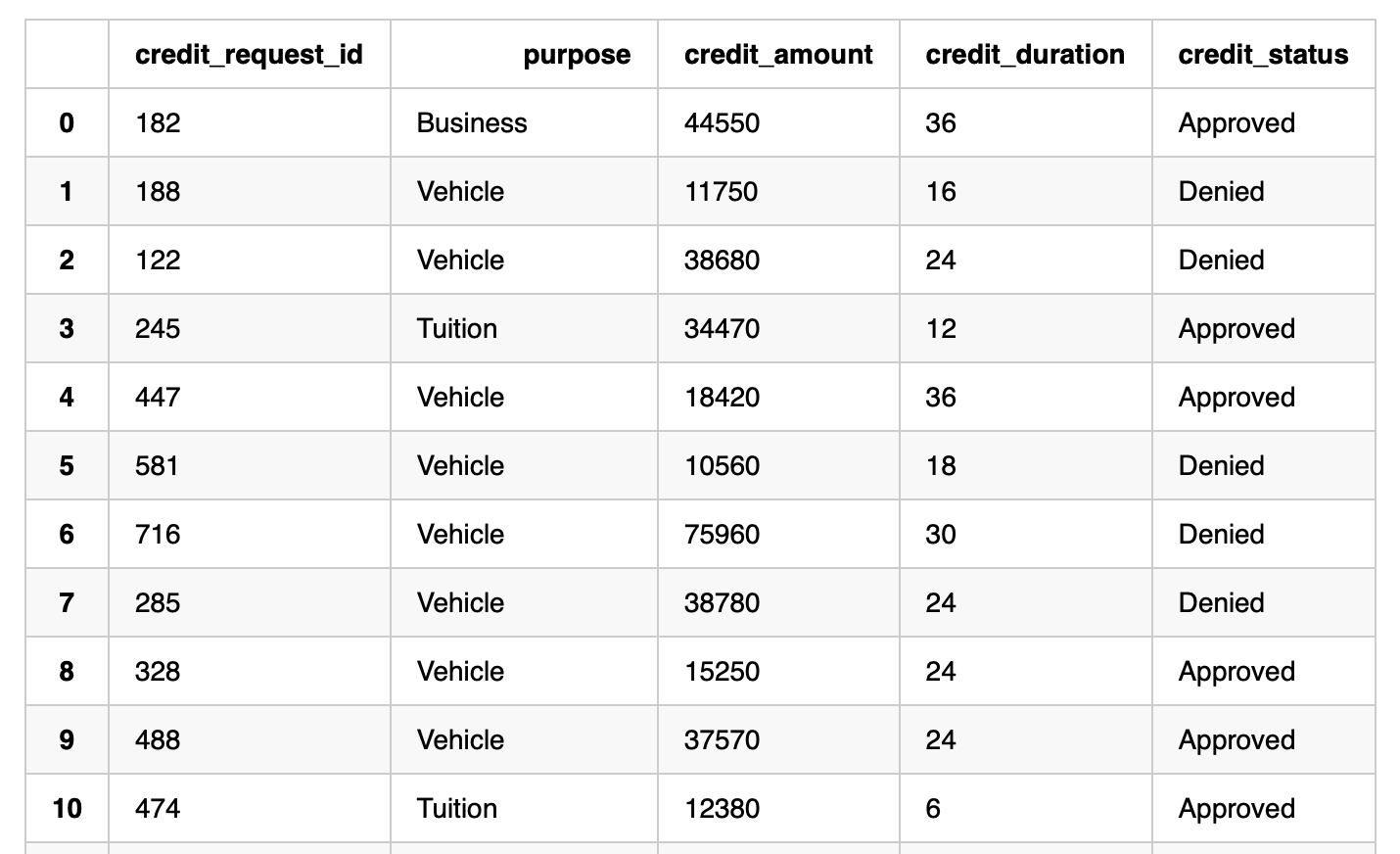
5. Inference in Lakehouse

In the following example, we want to process 60 pending credit requests and evaluate whether the loans should be approved. The data is shown below:

df_cred_req = session.table("CREDIT_REQUESTS")

df_cred_req.toPandas()

df.info()

6. Develop Scoring Function

When Zettabank receives credit requests, we want to write a function that can be called via tasks to score incoming micro-batch requests.

The Python function will first use Zettapark API to build the model's input features for scoring.

from clickzetta.zettapark.functions import col, when def process_credit_requests_fn (session, credit_requests: str, credit_assessment: str) -> int: # Build model input features using Zettapark API direct encoding. df_cred_req = session.table(credit_requests).select( col("CREDIT_REQUEST_ID"), col("PURPOSE"), when(col("PURPOSE") == "Consumer Goods", 1) .when(col("PURPOSE") == "Vehicle", 2) .when(col("PURPOSE") == "Tuition", 3) .when(col("PURPOSE") == "Business", 4) .when(col("PURPOSE") == "Repairs", 5) .otherwise(0).alias("PURPOSE_CODE"), when(col("QUALIFICATION") == "unskilled", 1) .when(col("QUALIFICATION") == "skilled", 2) .when(col("QUALIFICATION") == "highly skilled", 3) .otherwise(0).alias("QUALIFICATION_CODE"), when(col("OTHER_PARTIES") == "Guarantor", 1) .when(col("OTHER_PARTIES") == "Co-Applicant", 2) .otherwise(0).alias("OTHER_PARTIES_CODE"), when(col("OTHER_PAYMENT_PLANS") == "bank", 1) .when(col("OTHER_PAYMENT_PLANS") == "stores", 2) .otherwise(0).alias("OTHER_PAYMENT_PLANS_CODE"), when(col("HOUSING") == "rent", 1) .when(col("HOUSING") == "own", 2) .otherwise(0).alias("HOUSING_CODE"), when(col("ASSETS") == "Vehicle", 1) .when(col("ASSETS") == "Investments", 2) .when(col("ASSETS") == "Home", 3) .otherwise(0).alias("ASSETS_CODE"), when(col("SEX") == "M", 1) .otherwise(0).alias("SEX_CODE"), when(col("MARITAL_STATUS") == "Married", 1) .when(col("MARITAL_STATUS") == "Single", 2) .otherwise(0).alias("MARITAL_STATUS_CODE"), col("CHECKING_BALANCE"), col("SAVINGS_BALANCE"), col("AGE"), col("JOB_HISTORY"), col("CREDIT_SCORE"), col("CREDIT_DURATION"), col("CREDIT_AMOUNT"), col("RESIDENCE_SINCE"), col("INSTALLMENT_COMMITMENT"), col("NUM_DEPENDENTS"), col("EXISTING_CREDITS") ) # Call UDF to score previously read existing credit requests input_features = [ 'PURPOSE_CODE', 'QUALIFICATION_CODE', 'OTHER_PARTIES_CODE', 'OTHER_PAYMENT_PLANS_CODE', 'HOUSING_CODE', 'ASSETS_CODE', 'SEX_CODE', 'MARITAL_STATUS_CODE', 'CHECKING_BALANCE', 'SAVINGS_BALANCE', 'AGE', 'JOB_HISTORY', 'CREDIT_SCORE', 'CREDIT_DURATION', 'CREDIT_AMOUNT', 'RESIDENCE_SINCE', 'INSTALLMENT_COMMITMENT', 'NUM_DEPENDENTS', 'EXISTING_CREDITS'] df_assessment = df_cred_req.select( col("CREDIT_REQUEST_ID"), col("PURPOSE"), col("CREDIT_AMOUNT"), col("CREDIT_DURATION"), when(col("CREDIT_SCORE") > 600, "Approved").otherwise("Denied").alias("CREDIT_STATUS")) df_assessment.write.mode("overwrite").saveAsTable(credit_assessment) # The function returns the number of credit requests evaluated. return df_assessment.count()

7. Call the Scoring Function

process_credit_requests_fn (session, "credit_requests", "credit_assessments")

session.table("credit_assessments").toPandas()

Appendix: