Data Freshness and Dynamic Tables

Data freshness measures the latency between when data is generated and when it becomes available for querying. Hourly refresh is enough for weather forecasts, while a nuclear power plant control system needs millisecond-level response. Freshness requirements can differ by orders of magnitude across scenarios.

Designing a data processing pipeline starts with defining what is "fresh enough" instead of always chasing the lowest latency. The test is simple: If data arrives N minutes late, does it cause measurable business loss? If not, the target is sufficient. Changing a dashboard from refreshing every 5 seconds to every 5 minutes may not affect decision quality, but it can change system architecture and operations cost by orders of magnitude.

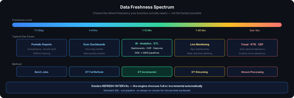
Freshness Is a Spectrum, Not a Switch

"Real-time" and "offline" are legacy labels that reduce a continuous spectrum to two categories. In practice, freshness looks like this:

Freshness Level	Typical Interval	How Data Is Refreshed
Daily	T+1	Batch jobs run at night, full recomputation
Hourly	Every 1–4 hours	Scheduled jobs, incremental or full computation
Minute-level	Every 1–15 minutes	Detect data changes and refresh incrementally on demand
Second-level	1–30 seconds	Event-driven, continuous incremental refresh
Sub-second	< 1 second	Per-event persistent processing

The further right you go, the lower the latency and the higher the cost. The engineering question is: which frequency band does your scenario actually need?

The Widespread Misuse of the "Real-Time" Label

Many scenarios labeled "real-time" do not actually require second-level or sub-second latency from a business perspective. An IDC 2025 industry survey found that 63% of data processing scenarios only need minute-level freshness to meet business requirements. Core report delivery can use minute-level freshness as the standard, including fault recovery time. Marketing activity analysis can explicitly target minute-level freshness. BI dashboards that refresh within 1 to 15 minutes do not degrade decision quality.

Behind this is a common pattern: analytical workloads are consumed by people. Reading dashboards, understanding trends, and making decisions already takes minutes to hours. Whether data is available in 5 minutes or 5 seconds often makes little difference to the final decision, but it can change system architecture and operations cost by orders of magnitude.

In production environments, the bottleneck in end-to-end latency is often not the processing engine, but the upstream collection frequency and downstream consumption pace. Extracting data from business systems has its own latency, such as CDC log polling or file arrival cycles. After results are pushed to dashboards, users may check them only every half hour. Running the middle processing layer at second-level latency, while upstream and downstream stages remain slower, adds cost without corresponding value.

Consumption patterns also determine the effective upper bound on freshness. If the result goes into a weekly email report that is read once a day, minute-level refresh is meaningless; T+1 is sufficient. If the result serves an automated decision API embedded in an operations system, freshness requirements are determined by the API call frequency. If the API is called every 5 minutes, data refreshed within 10 seconds adds no value. BI tool connection methods also affect freshness: direct queries can retrieve the latest data each time, while scheduled imports are limited by import frequency. Derive freshness targets backward from the consumption end. First ask how the data is ultimately used, then ask how fast the processing pipeline should be.

Another commonly overlooked factor: stream processing often remains in production because of stateful semantics, not because of latency. Exactly-once semantics, out-of-order event correction, and complex event pattern matching are the capabilities that stream engines are hard to replace for. Many streaming jobs exist to unify stream and batch architectures or reuse resources, not because the business requires sub-second latency.

The IDC 2025 industry survey showed that 63% of data processing scenarios only need minute-level freshness. The engineering community is moving in the same direction. Multiple engines are converging on the same goal: let users declare how fresh the data needs to be, and let the engine decide whether to use batch or stream processing. Flink Materialized Tables, Snowflake Dynamic Tables, and Databricks DLT all follow this pattern. This is not a coincidence; it is a common answer to the same engineering constraints.

Three Computational Paradigms: How Incremental Computing Changes Batch and Stream Processing

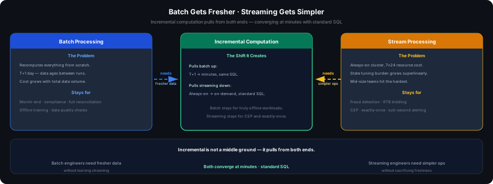
Incremental computing is not just "a third option between batch and stream." It changes both batch and stream processing, pulling them toward the middle.

Batch Processing: Better Freshness Without Learning Stream Processing

The core problem with batch processing is not correctness. Batch processing is often the most accurate way to compute. The problem is that freshness cannot keep up with business needs. A dashboard that delivers T+1 data shows yesterday's data. Market changes this morning may not be analyzed until this afternoon.

The traditional path is to learn stream processing: build a stream processing pipeline, deploy a persistent cluster, and understand watermarks, windows, and triggers. For data teams that primarily use SQL, this is a large shift in toolchain and skills.

Incremental computing offers an alternative path: you do not need to learn stream processing or change the toolchain. Declare REFRESH INTERVAL 5 MINUTE in the same standard SQL, and the batch processing pipeline changes from T+1 to minute-level freshness. For most batch processing scenarios that only need minute-level freshness, this is sufficient.

Many teams do not start from stream processing at all; they start from daily batch processing. When the business starts saying that yesterday's data is not enough, the options often become either accepting the status quo or introducing an entire stream computing system. Stream computing means a new language, new operations, and new team skills. Incremental computing is not just cheaper than stream processing; it also makes possible scenarios that were never built as real-time pipelines because the barrier was too high.

Stream Processing: Simpler Operations Without Losing Real-Time Capability

The core problem with stream processing is not speed. It is fast enough. The problem is that architectures designed for second-level latency are often used for scenarios that only need minute-level freshness.

Persistent clusters occupy resources 24/7. State backend tuning requires dedicated expertise. Checkpoint and backpressure tuning become harder as the number of jobs grows. The operational burden is especially difficult for mid-sized teams. Very large organizations can maintain dedicated Flink platform teams and reuse nighttime idle resources through mixed deployment, reducing per-job cost. Teams with very few jobs can manage the native operational complexity. Teams in the middle suffer most: the number of jobs is too high for simple operations, but the scale is not large enough to justify a dedicated stream computing platform team. Every new business line adds another layer of operational burden.

The consequence is not only harder operations. A new business line that only needs minute-level freshness may choose not to build the pipeline if it must bear the TCO and specialist requirements of a persistent streaming cluster. The scenario may have value, but the barrier blocks it. Incremental computing opens up scenarios that would otherwise never be built.

Cloud-managed Flink reduces visible operational burden but does not remove the root cause. Resources are still persistent, which means paying even during low-peak periods. New business lines still need to decide whether the cost is worth it.

When a pipeline simply processes data from ODS to DWD for downstream dashboards, and a 3-minute delay is acceptable, a 24/7 persistent cluster may not be worth the cost.

Incremental computing offers a simpler option: scenarios that require sub-second latency, such as anti-fraud, real-time bidding, and CEP, can keep stream processing. Scenarios that only need fresher queryable data can use declarative SQL. There is no need to manage state, understand checkpoints, or respond to backpressure at night. Set the refresh frequency and let the engine do the work.

What Will Stay, What Will Migrate

Paradigm	Scenarios That Will Stay in Original Paradigm	Scenarios That Will Migrate to Incremental Computing
Batch processing	Month-end reconciliation, compliance auditing, scenarios requiring full-data validation	BI dashboards, operational analysis, marketing reports, daily ETL
Stream processing	Anti-fraud interception, RTB bidding, sub-second alerts, stateful CEP requiring exactly-once	CDC ingestion to data warehouse, feature engineering, real-time big screens, minute-level data warehouses

Incremental computing is not inserting a middle option between batch and stream. It redefines both lines: batch processing is pulled up to minute-level freshness, and the portion of stream processing used only for minute-level freshness is pulled down to declarative SQL. Both ends converge toward the middle. Switching from persistent computing to on-demand refresh changes cost by orders of magnitude, not by a marginal percentage.

How Singdata Lakehouse Implements It

Singdata Lakehouse implements tiered freshness through two core capabilities:

Data ingestion: Continuously ingest data through real-time sync tasks (database CDC) or Pipe (Kafka / object storage), with latency options from seconds to minutes.

Dynamic Table: Define multi-level freshness using standard SQL. The REFRESH INTERVAL clause controls the refresh frequency; the engine adaptively chooses between full or incremental execution underneath. See Dynamic Table.

CREATE DYNAMIC TABLE dws_sales_dashboard REFRESH INTERVAL 5 MINUTE VCLUSTER DEFAULT AS SELECT ...; -- Same standard SQL as batch processing

REFRESH INTERVAL 5 MINUTE tells the engine that data should be no more than 5 minutes behind. The engine decides whether to use incremental or full execution for each refresh.

How to Determine What Freshness Level a Scenario Needs

First, and most critical: do you need computational semantics, or data freshness?

These two types of requirements are fundamentally different. They are not simply faster-versus-slower trade-offs.

If the business requires exactly-once guarantees, out-of-order event correction, or complex event pattern matching, such as the same account logging in from three locations within 10 minutes, that is a computational semantics problem. The core requirement is not how quickly data is available, but that the computation must not produce errors or miss data. Use stream processing; incremental computing is not a substitute.

If you simply want data to be available as soon as possible so dashboard numbers can catch up with recent events, that is a freshness problem. Use incremental computing, declare the refresh interval you need, and leave the rest to the engine.

After confirming it is a freshness problem, ask two more specific questions:

Who are the data consumers?

If they are people using dashboards, reports, or BI analysis, minute-level freshness is almost always sufficient. The pace of human decision-making determines the effective upper bound on data freshness. If the consumer is an automated decision system, such as anti-fraud interception or a bidding engine, then second-level or sub-second freshness may be required. At that point, you are usually back to a computational semantics problem.

Can the upstream and downstream of the pipeline support how fast you want to go?

If the source data is an hourly file, processing the middle layer at second-level frequency has no value. If results are pushed to a weekly report viewed once a week, second-level refresh also has no value. Freshness is determined by the slowest link in the pipeline; accelerating only one middle segment is wasteful.

Freshness requirements within the same business are layered.

A data dashboard may require minute-level freshness, a trending leaderboard may require hourly freshness, and compliance reports may require daily freshness. These requirements often coexist in the same business. Using one stream processing architecture for all layers means paying the cost of the strictest requirement for every scenario. Layered configuration, with different Dynamic Tables using different refresh intervals, is more economical and easier to maintain than a one-size-fits-all approach.