
Cost-Effective Alternatives to Databricks and Snowflake: A Buyer's Evaluation Framework
A buyer's framework for evaluating cheaper Databricks and Snowflake alternatives: diagnose your bill, match pricing models to workload shape, assess lock-in and TCO, and validate with a PoC checklist.
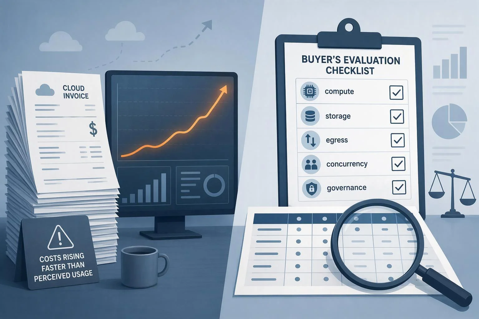
Your Databricks or Snowflake bill is growing faster than the workloads it pays for, and the renewal quote has arrived with a number you cannot explain to finance. The obvious next step is to shop for a cheaper platform. That step usually fails, because the platforms you are comparing do not meter the same thing, and the workload that dominates your bill may not be the workload you think it is.
This article is a buyer's evaluation framework, not a ranking. It works through five questions in order: how your current bill is actually generated, which pricing model fits your workload shape, what lock-in survives an open table format, what a defensible total cost of ownership (TCO) model contains, and what capability you give up when you move. Vendor-published savings figures appear here only as claims to validate in your own environment, never as established facts.
Why Your Bill Grows When Usage Feels Flat
Perceived usage and billed cost diverge because most platforms meter resources held open, not work completed. A dashboard that loads in the same two seconds every morning can cost four times as much this quarter as last, with no change in query volume, if the warehouse behind it was resized or left running. Before comparing vendors, establish where the growth sits in your own account. Four places account for most of it: always-on compute, oversized compute, interactive compute doing scheduled work, and storage plus egress.
Snowflake Gen1 standard warehouse credit rates, as published in the warehouse-size table. Credits per hour double with each size step; the per-second column is the hourly rate divided by 3,600 and is rounded in the source. Rates are per running hour and exclude the 60-second minimum charged on each start or resume, cloud services above the 10% daily threshold, storage and egress.
Snowflake bills compute credits per second with a 60-second minimum, and warehouse size sets the multiplier. An X-Small warehouse consumes 1 credit per hour; each step up doubles it, so 6X-Large consumes 512 credits per hour (Snowflake warehouse sizes). A warehouse that runs continuously at 6X-Large bills 512 credits for every hour of the month, whether or not queries arrive. The 60-second minimum compounds the problem for short, frequent queries: a warehouse resumed for a 3-second query still bills a full minute at its size multiplier.
Cloud services credits are a separate line. Snowflake bills cloud services consumption only to the extent it exceeds 10% of daily warehouse compute credits, calculated daily in UTC (Snowflake compute cost documentation). On a low-compute day, that adjustment is small in absolute terms, so metadata-heavy periods can produce a cloud services charge that looks disproportionate to the warehouse activity beside it.
Databricks meters in DBUs and separates compute types. Its own cost guidance states that non-interactive workloads cost significantly less on job compute than on all-purpose compute, and that a Databricks SQL warehouse is the most cost-efficient engine for interactive SQL (Databricks cost optimization best practices). The common failure is a scheduled pipeline running on an interactive all-purpose cluster because that is where it was developed. Idle clusters and GPU instances attached to workloads that do not use GPU-accelerated libraries are the other recurring leaks the same guidance flags.
Diagnose before you shop. Pull 90 days of billing data and attribute compute to workload class: scheduled ETL, interactive BI, ad hoc exploration, and always-on serving. If the growth sits in a workload class that a different metering model would price better, an alternative is worth evaluating. If it sits in a warehouse nobody turned off, the cheapest fix is a configuration change, and no migration will beat it.
Evaluation Criteria: How to Compare Any Alternative
Five criteria decide whether an alternative is genuinely cheaper for you, and each gets its own treatment below. First, pricing model fit: does the vendor meter provisioned capacity, consumed resources, or scanned data, and does that match how your workload arrives over time? Second, lock-in: what stays tied to the platform after your data is in an open table format? Third, TCO: what does the full line-item cost include beyond compute? Fourth, migration and operational risk: what must be rebuilt, retested, and staffed? Fifth, capability coverage: which governance, machine learning, and streaming functions must reach parity before cutover?
Order matters. A platform that wins on price per credit but loses on criteria two through five is not cheaper; it has moved cost from the invoice to the engineering budget. Score each candidate against all five before requesting a quote, and treat any vendor response that addresses only the first as incomplete.
Pricing Model Fit: Matching Metering to Workload Shape
The candidate categories meter compute in materially different ways, and the right choice depends on whether your demand is steady, spiky, or batch. The table below summarizes how each meters compute; list prices change and regional pricing differs, so confirm current rates on each vendor's pricing page before modeling.
Platform | Metering unit | Granularity and floors | Notable mechanics |
|---|---|---|---|
Snowflake | Credits | Per second, 60-second minimum | Size multiplier from 1 credit/hour (X-Small) to 512 (6X-Large); cloud services billed above 10% of daily warehouse compute |
Databricks | DBUs | Per second | Jobs Compute priced below All-Purpose Compute; SQL warehouses include Photon by default; spot instances for eviction-tolerant work |
BigQuery | Bytes scanned (on-demand) or slot-hours (capacity) | On-demand: up to 2,000 slots per project; capacity: 50-slot reservation minimum | Switchable between models at any time; autoscaling or committed slots |
Redshift Serverless | RPU-hours | Per second, 60-second minimum | Entry point advertised from $1.50/hour; reservations advertised up to 45% for three years |
Microsoft Fabric | Capacity units (F SKUs) | Per second, one-minute minimum via Azure | F capacities via Azure with optional yearly reservation; P capacities require an active Enterprise Agreement |
Amazon EMR | Instance-hours plus EMR uplift | Per second, one-minute minimum | EMR price added to EC2 and EBS cost; Spot instances advertised up to 90% below On-Demand |
Trino / Starburst, Dremio | Self-managed infrastructure, or engine runtime | Varies by deployment | Dremio meters engine size × minutes running in DCUs, with infrastructure included |
BigQuery's two models behave very differently. On-demand bills bytes processed in the columns you select, even with a LIMIT on results, so partitioning and clustering directly reduce cost; capacity-based billing allocates slots with a 50-slot minimum and increments of 50, and you can switch between the two at any time (BigQuery pricing, reservations overview). Redshift Serverless bills RPU-hours per second with a 60-second minimum, and its reservations are metered per second while billed hourly (Redshift Serverless billing, Redshift pricing).
Fabric's capacity model is a licensing decision as much as a pricing one. F capacities are purchased through Azure and billed per second with a one-minute minimum, with optional yearly reservations; P capacities are available only to customers holding them on an active Enterprise Agreement with monthly or yearly billing (Fabric licenses). EMR adds its per-second, one-minute-minimum charge on top of the underlying EC2 and EBS cost, and Spot capacity is available at a discount for workloads that tolerate eviction (EMR pricing).
Map workload shape to model plainly. Steady, high-concurrency BI favors capacity commitments, because predictable baseline demand is what commitments discount. Spiky ad hoc exploration favors consumption pricing, because you pay for what runs and nothing for the quiet hours. Eviction-tolerant batch favors spot-backed engines, where the discount is compensation for interruption risk. Self-managed engines shift the infrastructure line into your own cloud bill, which can be cheaper at scale and more expensive in labor.
Open Table Formats and What Lock-In Actually Remains
Open table formats solve data portability. They do not, by themselves, solve platform portability, and buyers routinely conflate the two. The distinction is worth stating precisely before you accept "open format" as an answer to lock-in.
What the formats provide is real. Delta Lake documents compute engines including Spark, PrestoDB, Flink, Trino, Hive, Snowflake, Google BigQuery, Athena, Redshift, and Azure Fabric, and its UniForm capability lets Iceberg and Hudi clients read Delta tables (delta.io). The Iceberg specification defines table metadata, snapshots, manifests, and schema evolution in an open, versioned format that any conforming engine can read (Iceberg table spec). Your Parquet files and table metadata are not trapped.
What stays tied sits above the files. The catalog and metastore determine where tables live and who can find them; the Iceberg spec states that when the location field is absent, the table location must be provided and that catalogs should provide a table's location, which makes the catalog a functional dependency rather than a convenience. Governance layers, access-control models, and audit trails are platform-specific even when they govern open tables. Proprietary optimizations such as query accelerators, caching layers, and vendor-tuned runtimes do not travel with the data. Managed-service operational tooling, from cluster autoscaling to job orchestration, is not part of any format specification.
Use a two-column mental model. Data portability asks whether another engine can read your tables tomorrow; the answer is usually yes. Platform portability asks whether you can run the same pipelines, under the same governance, with the same operational tooling, on a different platform next quarter; the answer depends on how much of your logic lives in the catalog, the governance layer, and vendor-specific SQL. Before committing, inventory which of those three your critical pipelines depend on.
Building a TCO Model That Survives Scrutiny
A TCO model that survives finance review has seven line items, and compute is only the first. Build it in a spreadsheet with a stated assumption for each line, and keep those assumptions visible so a reviewer can challenge them individually.
Illustrative arithmetic only, not observed data or a benchmark. Inputs are stated assumptions chosen to show the calculation: $40,000/month current compute and storage, a 40% lower compute rate, 1,200 engineering hours at $120/hour, $30,000 training and tooling, three months of dual running at half the old platform's cost, and $4,000/month added egress. Bars show the first-year cash effect of each line; the net is a $90,000 first-year cost. Substitute your own figures.
Compute. Model at production scale and concurrency, not at pilot volume. Separate the always-on baseline from peak.
Storage. Include active and long-term tiers, plus any copies created by replication or materialized views.
Egress and data transfer. Snowflake charges a per-terabyte fee when data moves to a different region on the same cloud or to a different cloud, at a rate that depends on the hosting region (Snowflake cost overview). AWS applies tiered data-transfer-out rates across services, with cross-region transfer billed separately (S3 pricing).
Governance and security tooling. Line-item the catalog, lineage, masking, and access-control products needed to reach parity.
Migration labor. Estimate engineering weeks for pipeline rewrites, SQL remediation, and testing, priced at fully loaded cost.
Ongoing operations. Include the headcount or managed-service fee required to run the new platform at your service levels.
Dual running and training. Budget the overlap period when both platforms bill simultaneously, plus retraining for analysts and engineers.
Illustrative worked example (inference, not observed data).Assume a team spends $40,000 per month on compute and storage today. A candidate platform quotes a 40% lower compute rate, implying $16,000 per month saved, or $192,000 per year. Assume the migration requires 1,200 engineering hours at a fully loaded $120 per hour, or $144,000, plus $30,000 in training and tooling. Assume dual running for three months at half the old platform's cost, or $60,000. Assume the new platform's egress profile adds $4,000 per month, or $48,000 per year. First-year net saving is $192,000 − $144,000 − $30,000 − $60,000 − $48,000 =−$90,000: the migration costs money in year one. The saving turns positive only in year two, and only if the compute discount holds at your actual workload. These figures are illustrative assumptions chosen to show the arithmetic; substitute your own.
One comparison error invalidates more business cases than any other: benchmarking a discounted incumbent renewal against a new vendor's list price. If your current contract carries a negotiated discount, compare the new vendor's discounted quote against it, on the same workload, for the same term.
Capability Trade-Offs: What You Give Up
Some alternatives are cheaper because they shift operational responsibility to you. That is a legitimate trade, not a hidden flaw, but it must be priced and staffed deliberately rather than discovered in month three.
Managed operations are the largest item. Snowflake positions itself as a fully managed product that handles infrastructure management (Snowflake pricing). A self-managed Trino deployment, by contrast, is a distributed SQL query engine (Trino overview); running it yourself means you install, size, upgrade, and secure it. The infrastructure saving is real; so is the platform engineering headcount that replaces it.
Governance and catalog layers rarely transfer intact. Access policies, row-level rules, lineage, and audit history are configured per platform, and rebuilding them is migration work with a security review attached. Machine learning tooling is similarly platform-bound: Databricks maintains separate runtimes optimized for data engineering and for machine learning tasks, with curated library sets and a regular release cadence (Databricks cost optimization best practices). Reproducing that environment elsewhere is a project.
Streaming semantics deserve a specific test. Delta Lake documents unified batch and streaming with exactly-once semantics ingestion, and its cost guidance recommends balancing always-on against triggered streaming (delta.io, Databricks cost optimization). If your pipelines depend on those guarantees, verify equivalent behavior under failure and restart on the target platform before cutover, not after.
Write down what you are giving up, in the same document as the savings. A trade you chose and staffed is a strategy; the same trade discovered late is an incident.
Reading Vendor "X% Cheaper" Claims
Vendor comparison pages are marketing documents with a methodology attached, and the methodology is where the claim lives or dies. Common patterns include comparing list price to list price when you pay a negotiated rate, benchmarking a best-case workload against an average one, and excluding labor and egress from the total. None of these is necessarily dishonest; all of them change the answer for your environment.
Ask six questions of any savings claim before it enters your business case. What exact workload was measured, at what data volume and concurrency? What baseline was it compared against, and was that baseline a list price or a discounted contract? Which cost categories are excluded, specifically labor, egress, storage, and governance tooling? What commitment term is assumed, and what happens to the price at renewal? Was the comparison run on the vendor's hardware and configuration, and can you reproduce it? Does the claim describe a benchmark result or a customer outcome, and if the latter, what was that customer's starting configuration?
A claim that survives all six questions is a hypothesis worth testing in your own proof of concept. A claim that cannot answer them is a data point about the vendor's marketing, not about your cost.
Validating Before You Commit: A PoC Acceptance Checklist
A proof of concept should produce evidence you can write into a contract, not a demo you remember favorably. Define acceptance criteria before the vendor starts, and make each one measurable.
Representative query mix and concurrency. Run your actual top queries by frequency and cost, at production concurrency, not a synthetic benchmark.
Cost per workload at production scale. Measure cost per pipeline run and cost per dashboard load at full data volume, and compare against the same measures on your current platform.
Governance and access-control parity. Demonstrate that every role, row-level rule, and masking policy in production has an equivalent, tested configuration.
Migration of the hardest tables and pipelines. Pick the pipelines with the most vendor-specific SQL, not the easiest ones.
Egress volumes. Measure actual data-transfer volume and cost for your real consumption patterns, including cross-region reads.
Operational runbooks. Confirm that failure recovery, scaling, and on-call procedures are documented and tested by your own team.
A measured exit path. Export your data and metadata from the new platform once, timed and documented, so the exit cost is known rather than assumed.
Each item becomes a contract clause with a defined pass threshold. If a vendor will not accept a measurable threshold on cost per workload and governance parity, that refusal is itself information.
Who Should Choose Which
Use these profiles as a starting filter, then validate with the criteria above. Each mapping names where the option loses, because a recommendation without its failure mode is not usable.
Steady, BI-heavy estates with predictable baseline demand should evaluate capacity commitments, where BigQuery slot reservations and Redshift Serverless reservations discount predictable load. They lose flexibility: commitments are sunk if demand falls.
Spiky exploratory analytics with long quiet periods should evaluate consumption pricing such as BigQuery on-demand or Snowflake per-second credits. They lose predictability, and a single unpartitioned query can dominate a month.
Spark-centric machine learning shops should weigh the cost of leaving Databricks against the value of its ML runtimes and job-versus-all-purpose separation. They lose the integrated runtime if they move, and must rebuild it.
AWS-native teams should evaluate Redshift Serverless and EMR, which bill into an existing AWS account and reuse existing commitments. They lose cross-cloud flexibility and inherit AWS regional pricing.
Microsoft-centric teams already holding an Enterprise Agreement should evaluate Fabric F capacities, which bill per second through Azure. They lose the option of a non-Microsoft stack without a licensing review.
Cost-sensitive teams willing to self-manage should evaluate Trino or Starburst on their own infrastructure, or Dremio's DCU model. They take on platform engineering, and should staff it before signing.
Teams evaluating unified lakehouse platforms should add Singdata to the shortlist as one option in that category, alongside the criteria above. Singdata describes a single-engine architecture and incremental compute, and publishes performance and cost figures on its site; treat those as vendor-reported claims to reproduce in your own PoC rather than as established results. The evaluation questions do not change: measure cost per workload at your scale, test governance parity, and time the exit.
FAQ
Do open table formats eliminate lock-in? No. They make the data portable; they do not make the platform portable. Your catalog, governance layer, and managed tooling stay behind, as the lock-in section explains.
Does a cheaper list price guarantee a lower TCO? No. Engineering labor, egress, and dual-running during cutover often outweigh the compute difference. Build the line-item model before you compare quotes.
Can migration be staged? Yes. Offloading one workload class — typically interactive BI or ad hoc exploration — is a lower-risk first step than a full migration, and it gives you measured cost data for the rest of the decision.