
Automating Weekly Data Forecasting: A Pipeline Design and Acceptance Guide
Design a reliable automated weekly forecasting pipeline: enforce cutoff and restatement rules, use rolling-origin backtests, govern metric definitions, and audit overrides.
Introduction
A weekly forecast is a recurring production commitment. Someone downstream — a replenishment planner, a capacity scheduler, a finance analyst — expects a number every week, for every series in scope, by a stated time, and will act on it. That commitment is what makes automation hard. Fitting a model once is a modeling exercise; running it fifty-two times a year against data that keeps arriving late, definitions that keep changing, and exceptions that keep appearing is an operations problem.
The central claim of this guide is that reliability comes from how the pipeline handles time and how it is governed, not from model choice alone. Two pipelines using the same model can differ enormously in trustworthiness depending on whether features are rebuilt as of the cutoff, whether backtests mimic the real forecast origin, whether metric definitions are versioned, and whether overrides leave an audit trail. Model selection matters, but it sits downstream of those decisions.
The sections that follow cover the weekly operating contract, the staged pipeline and its checkpoints, rolling-origin backtesting, accuracy metric selection and the documented limits of percentage errors, semantic consistency of the forecasted quantity, exception routing and override audit, and a testable acceptance checklist. The basis is design reasoning plus published forecasting methodology, principally Hyndman and Athanasopoulos's Forecasting: Principles and Practice (3rd edition, FPP3), together with established data warehousing practice on bi-temporal data. No claim here rests on a deployment we observed.
What "Weekly" Operationally Requires
Before any model runs, the weekly cycle needs four parameters written down and enforced by the pipeline. Each is easy to leave implicit and expensive to discover later.
Data cutoff. The latest timestamp of source data a run is permitted to use. A cutoff is a timestamp, not a date. "Data through Sunday" is ambiguous when a source system posts Sunday transactions at 03:00 Monday; "data with arrival timestamp at or before Monday 02:00" is not.
Publication deadline. When the forecast must be available to consumers. The interval between cutoff and deadline is the processing budget, and it has to cover ingestion, validation, feature construction, model execution, reconciliation against the prior vintage, and any human review gate — not just model runtime.
Late-arriving data window. How long after a period closes the pipeline will still accept corrections to that period. This determines whether last week's forecast is treated as final or provisional.
Restatement policy. What happens when late data arrives inside the window: whether the prior published forecast is revised, how the revision is labeled, and who is notified. Without a stated policy, revisions happen ad hoc and consumers cannot tell a correction from a model change.
Effective date versus arrival timestamp
The distinction that makes restatement tractable is the one Roelant Vos sets out in his paper on bi-temporal backdated adjustments. Two time attributes are tracked separately: the load date/time stamp, recording when a row arrived in the warehouse, and the change date/time stamp, the business effective date supplied by the source system. A record can arrive in February and be effective from the previous December. Vos's worked example is a sales figure for June reported as $120k in November and $125k in December — the same business period, two different answers, because a backdated adjustment arrived between the two readings.
Kimball's Type 2 slowly changing dimension pattern encodes the same idea with begin- and end-effective datetimes plus a current flag, preserving history rather than overwriting it. For a forecast pipeline the consequence is direct: every published forecast must record which data vintage produced it — the arrival-time state of the inputs at the cutoff — so that a later restatement can be explained rather than merely observed. Vos frames this as a trust problem: consumers ask why a past figure changed, and a deterministic, replayable process is what lets you answer.
The ISO week boundary
Week numbering is a concrete calendar constraint that automation must settle before it can key on weeks. ISO 8601 weeks begin on Monday, and an ISO year contains 52 or 53 weeks. The ISO calendar reference notes that an ISO calendar year is long — 53 weeks — if and only if the corresponding Gregorian year begins on a Thursday, or is a leap year beginning on a Wednesday; long years in the current cycle include 2004, 2009, 2015, 2020 and 2026. A pipeline that assumes 52 weeks per year, or that keys on calendar year rather than ISO week-year, will misalign series at year boundaries and produce a spurious step change in any weekly aggregate. Decide the rule — ISO week-year with an explicit handling for week 53 — and encode it once, in the date dimension, rather than in each downstream query.
Staging the Recurring Pipeline and Its Checkpoints
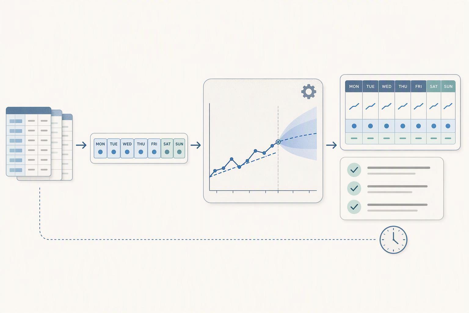
The recurring pipeline has seven stages. The value of naming them is that each transition gets a checkpoint with a pass/fail condition, so a failed run stops at a known place instead of publishing a plausible-looking number.
Ingest. Land source data with its arrival timestamp preserved. Checkpoint: expected partitions for the period are present and the row count is within a stated band of the trailing median. Fail means halt; a partial ingest that proceeds to forecasting produces a forecast of incomplete data.
Validate. Schema conformance, null rates on key fields, referential integrity against dimensions, and range checks on the target measure. Checkpoint: all validation rules pass, or failures are classified as blocking versus warning. Blocking failures halt; warnings route to the exception queue described below.
As-of feature build. Reconstruct features from the data vintage available at the cutoff. This is the stage where silent leakage enters automated runs. If features are read from current-state tables, a run that executes on Tuesday will see Monday's corrections to last week's actuals, and the model will be trained and scored on information no real forecast could have had. The feature build must filter on arrival timestamp — the load-date axis — not on business effective date alone. Checkpoint: a reproducibility test confirms that rebuilding features for a past cutoff from the retained raw history returns the same values as the original run.
Forecast. Execute the model or model set per series. Checkpoint: every series in scope has an output, and outputs fall within configured plausibility bounds. A missing series is a failure, not a gap to be filled downstream.
Reconcile. Compare the new run against the prior published vintage. Classify each material difference as either an expected restatement — explained by late data inside the window, with the contributing records identified — or an anomaly requiring review. Checkpoint: every difference above the materiality threshold carries a classification. This stage is what turns restatement from a surprise into a documented event.
Publish. Write the forecast with its vintage identifier, model version, metric-definition version, and run metadata. Checkpoint: the published artifact is complete and the vintage is recorded. Publication should be atomic — a partially published week is worse than a delayed one.
Monitor. Track realized accuracy as actuals arrive, and track input distribution shifts. Checkpoint: realized error is computed at each horizon as actuals land, and drift signals are raised for investigation. Note that an input shift is an investigation signal, not automatic grounds for retraining; the drift literature distinguishes detecting that a distribution changed from establishing that the model's error changed with it.
Human gates belong at two transitions: between reconcile and publish when an anomaly is unclassified, and at monitor when a drift signal or accuracy breach exceeds a stated threshold. Everywhere else, the checkpoint should be machine-decidable. A gate that requires a person to approve routine runs reintroduces the manual dependency the automation was meant to remove.
Why Random Train/Test Splits Fail and How Rolling-Origin Backtesting Works
Random train/test splits are the default in much applied machine learning and they are wrong for forecasting evaluation. A random split assigns observations to training and test sets without regard to time, so the training set contains weeks that occur after weeks in the test set. The model is fitted on information from the future relative to the points it is scored on. No production run can do that: at the cutoff, the future has not happened. The result is an accuracy estimate that is optimistic by an amount nobody can quantify from the split alone.
Rolling-origin evaluation
FPP3 describes the correct procedure as time series cross-validation, also called evaluation on a rolling forecasting origin. A series of test sets is created, each consisting of observations that occur strictly after the corresponding training set. The origin — the point from which the forecast is made — rolls forward through the series, and accuracy is computed by averaging over the test sets. The earliest observations are not used as test sets because a forecast from a very short training history is not informative.
For multi-step horizons the procedure is modified. If the question is how well a method forecasts four weeks ahead, the test sets are constructed so that errors are measured at the four-step horizon rather than one step ahead, and the origin advances accordingly. FPP3 is explicit that one-step accuracy may not be the relevant question for a weekly planning cycle, where the decision typically depends on forecasts two to four weeks out.
Translating to the weekly setting
A backtest that is meant to support acceptance should mirror production on three dimensions:
The cutoff. Each simulated run uses only data with arrival timestamp at or before the historical cutoff, not all data effective before that date.
The horizon. Evaluate at the horizons the business actually consumes — commonly one to four weeks — and report accuracy per horizon, since error typically grows with lead time.
The vintage. Where the pipeline retains raw history with arrival timestamps, reconstruct the as-of state rather than reading current tables. This is the same requirement as the feature-build checkpoint, applied retrospectively.
The benchmark floor
FPP3 recommends comparing candidate methods against simple benchmarks — the mean method, the naïve method (last observed value), the seasonal naïve method (same week last season), and the drift method. A naïve forecast is optimal when the series follows a random walk, which makes it a meaningful floor rather than a formality. The acceptance rule is straightforward: a candidate method that does not beat seasonal naïve on the agreed metrics, evaluated on rolling origins, has not demonstrated value. Report the benchmark alongside the candidate in every backtest, not only at selection time.
Choosing Accuracy Metrics and MAPE's Pitfalls
Metric choice determines what the acceptance criteria actually reward, so it needs the same scrutiny as the model.
MAE is the mean absolute error, in the units of the series. Minimizing it targets the conditional median. RMSE is the root mean squared error; because errors are squared before averaging, large errors dominate, and minimizing it targets the conditional mean. If a large miss is disproportionately costly — a stockout, a missed capacity ceiling — RMSE reflects that preference better than MAE. If the cost is roughly linear in the size of the miss, MAE is the more faithful summary. Reporting both is cheap and reveals whether a method's advantage comes from typical accuracy or from avoiding tail errors.
MASE is the mean absolute scaled error. FPP3 defines it by scaling the forecast error by the average one-step naïve forecast error computed on the training data. Because numerator and denominator are on the original scale, the result is scale-free: a value below one means the forecast beat the average one-step naïve forecast on the training data, and above one means it did worse. This makes MASE usable across series with different units and volumes, and it anchors the comparison to a benchmark rather than to an arbitrary percentage.
Where MAPE fails
MAPE, the mean absolute percentage error, is the most commonly requested metric and the most frequently misapplied. FPP3 documents three problems with percentage-error measures:
They are infinite or undefined if any actual value in the period of interest is zero.
They take extreme values when actuals are close to zero.
They assume the unit of measurement has a meaningful zero point — the textbook's example is temperature, where a percentage error is meaningless because the zero is arbitrary.
For weekly series these are not edge cases. Intermittent demand, new product introductions, series with planned zero weeks, and low-volume SKUs all produce actuals at or near zero, and a single such week can dominate a MAPE average. A pipeline that accepts on MAPE will systematically favor methods that under-forecast small values, because under-forecasting a small actual produces a bounded percentage error while over-forecasting it produces a large one.
The practical rule is to select metrics per series type and state the aggregation rule explicitly. For high-volume, strictly positive series, MAPE may be acceptable as a secondary measure. For intermittent or low-volume series, use MAE, RMSE, or MASE. And distinguish per-series averaging from pooled error: averaging percentage errors across series weights each series equally regardless of volume, whereas a pooled error weights by magnitude. The two answer different questions, and the acceptance criterion should say which one it uses.
Keeping Metric Definitions and Semantics Consistent
A forecast is only comparable across runs if the quantity being forecast means the same thing each time. This sounds trivial and is one of the most common sources of unexplained accuracy shifts.
Consider a weekly revenue forecast. Does revenue count orders placed or orders shipped? Is it net of returns, and are returns attributed to the week of the original order or the week of the return? Which date attribute defines the week — order date, ship date, or invoice date? Each choice produces a different series, and a change in any of them changes the forecast without any change to the model.
The design response is one governed definition per metric: what is counted, which date attributes apply, which filters are included or excluded, and which source tables feed it. That definition is versioned. The forecast artifact records the definition version it used, exactly as it records the data vintage.
When a definition changes mid-stream, the consequence is a step change in apparent accuracy that is definitional, not model-driven. A pipeline that compares this week's realized error against last month's without checking the definition version will attribute the shift to the model and trigger an unnecessary investigation, or worse, a retraining cycle that chases a measurement artifact. The rule is that a metric-definition change triggers a backtest re-baseline: the historical evaluation is recomputed under the new definition before any comparison is made.
This is the same principle behind a shared semantic layer — one governed definition of each business metric, consumed by dashboards, models, and agents alike, rather than reimplemented in each. For forecasting it has a specific payoff: the series the model learns from, the series it is scored against, and the series the business reads in its reports are provably the same quantity. Where the platform provides a shared semantic layer, the forecast pipeline should read its target measure from it rather than from a private query, so that a definition change propagates to the model and the backtest together.
Routing Exceptions and Auditing Overrides
Automation does not eliminate exceptions; it changes how they are handled. The goal is to replace ad hoc manual rebuilds with structured review in which every deviation is classified, routed, and recorded.
Exception classes and routing
Class | Typical trigger | Routing |
|---|---|---|
Validation failure | Missing partition, null rate breach, schema mismatch | Halt run; auto-retry once on transient causes; notify data owner |
Reconciliation anomaly | Vintage-to-vintage difference above threshold, unexplained by late data | Hold publication; notify forecast owner for classification |
Accuracy breach | Realized error exceeds the configured threshold for a series | Publish with flag; open investigation; review at next cycle |
Upstream schema change | New or renamed column, changed data type | Halt run; route to engineering; require explicit approval to proceed |
The routing rule should be encoded, not remembered. Auto-retry is appropriate for transient infrastructure failures and inappropriate for data quality failures, where a retry simply reproduces the same bad input. Holding publication is appropriate when the anomaly is unclassified; publishing with a flag is appropriate when the forecast is usable but the series needs attention.
The override record
When a person adjusts a forecast, the adjustment must be recorded with enough detail to reconstruct what happened. The minimum fields are:
Who made the change and when.
Which series and which forecast week were affected.
The prior value and the new value.
The reason, drawn from a controlled list where possible.
The data vintage against which the override was made.
The effect on the published number, so downstream consumers can see the size of the manual contribution.
Replayability is the property that makes the record useful. If the next run can reconstruct the state before the override, it can distinguish a corrected input — where the source data itself was fixed and the override is now redundant — from a manual patch that still needs to be carried forward. Without that distinction, overrides accumulate silently and the published forecast drifts away from what the model produced, with no record of why.
An override without an audit trail converts an automated pipeline back into an untracked manual one. The schedule still runs, the artifacts still appear, but the number no longer has a traceable provenance, and the accuracy metrics measure a mixture of model output and undocumented human judgment.
A Testable Acceptance Checklist for a Weekly Forecast Pipeline
Each item below is a pass/fail condition a reviewer can check against the pipeline, its artifacts, and its logs. An item that cannot be checked is not yet satisfied.
Time contract
The cutoff timestamp, publication deadline, late-data window, and restatement policy are documented in one place and referenced by the pipeline configuration.
A test run confirms the pipeline refuses input with an arrival timestamp after the cutoff.
The ISO week rule, including week 53 handling, is encoded in the date dimension and used by every downstream query.
Reproducibility
Re-running a past week with the same inputs and vintage produces byte-identical or numerically identical output.
Raw source history with arrival timestamps is retained for at least the backtest window.
Leakage
Features are built by filtering on arrival timestamp, not on current-state tables; the feature-build query is reviewed and its filter is visible.
Backtests use rolling-origin construction only; no random or shuffled splits appear in evaluation code.
Backtests reconstruct the as-of vintage rather than reading current tables.
Benchmarks
Every backtest report includes naïve and seasonal naïve results alongside the candidate.
The candidate beats the benchmark on the agreed metrics at each reported horizon, or the shortfall is documented and accepted.
Metrics
Metric definitions are versioned, and each published forecast records the version used.
MAPE is excluded, or explicitly flagged, for series with zero or near-zero actuals.
The aggregation rule — per-series average versus pooled — is stated in the acceptance criteria.
Reconciliation
Every vintage-to-vintage difference above the materiality threshold carries a classification of expected restatement or anomaly.
Expected restatements identify the contributing late records.
Exceptions
Routing rules for each exception class are encoded and have been exercised in a test.
The override log contains all required fields for every manual adjustment in the review period, and a replay test confirms the pre-override state can be reconstructed.
Monitoring
Realized accuracy is computed at each horizon as actuals arrive, and the results are retained.
Drift signals raise an investigation task rather than triggering automatic retraining.
Conclusion
Weekly forecast automation succeeds when four things are designed together: the time contract that defines what data a run may use and when it must publish, the backtesting discipline that evaluates methods the way production will use them, the metric governance that keeps the forecasted quantity comparable across runs, and the exception audit that keeps human judgment traceable. Any one of these alone produces a pipeline that runs on schedule and still cannot be trusted.
The checklist in the previous section is the starting artifact. The practical next step is to run one historical week through the staged pipeline end to end — ingest, validate, as-of feature build, forecast, reconcile, publish, monitor — before automating the schedule. That single run exercises the cutoff enforcement, the vintage reconstruction, the reconciliation classification, and the publication record, and it surfaces the gaps that a design document will not.
Frequently Asked Questions
What is the difference between the data cutoff and the publication deadline?
The cutoff is the latest timestamp of data a run may use; the deadline is when the forecast must be published. The gap between them is the processing budget, and it must accommodate validation, feature construction, and reconciliation against the prior vintage — not just model runtime.
Can I use standard k-fold cross-validation for a weekly forecast?
Not for evaluation purposes. K-fold folds mix future and past observations, so the training set contains information the production run would not have had. Use rolling-origin (time series) cross-validation, in which every test set consists only of observations after its training set, as described in FPP3.
Why is MAPE a poor default metric for weekly forecasts?
MAPE is infinite or undefined when actuals are zero, extreme when actuals are near zero, and assumes a meaningful zero point. Intermittent and low-volume weekly series hit these conditions routinely. Use MAE or RMSE depending on whether typical or large errors matter more, and MASE when comparing across series with different scales.
How should late-arriving data be handled after a forecast is published?
The restatement policy should define the window in which late data triggers a revised forecast, and each published version should record its data vintage so revisions are explainable rather than silent. The reconcile stage classifies each revision as an expected restatement or an anomaly.
What should an override record contain?
At minimum: who made the change, when, which series and forecast week, the prior and new value, the reason, and the data vintage. The record must be replayable so the next run can distinguish a corrected input from a manual patch that still needs to be carried forward.
How do I know the automated pipeline is better than the manual process it replaced?
Score both on the same rolling-origin backtest with the same metrics. Where historical manual outputs were recorded, score them against realized actuals; where they were not, the baseline must be established prospectively before any improvement is claimed.