High-Frequency Data Modeling Performance Optimization: A Complete Guide
A step-by-step guide to high-frequency data modeling performance: set latency, freshness and cost targets, design grain and partitions, handle late data, and benchmark.
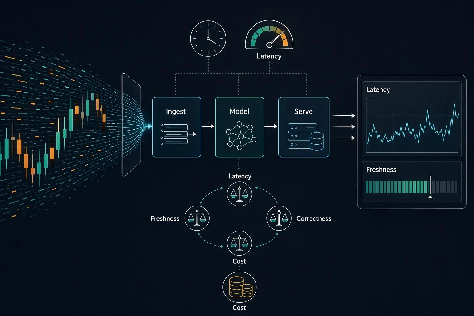
High-frequency data modeling performance is not a single tuning problem. It is a set of coupled trade-offs among latency, freshness, cost and correctness, and every change you make to one of them moves the other three. A schema that makes dashboards fast can make late-arriving events expensive to reconcile. A partition layout that cuts scan cost can multiply metadata overhead. A pre-aggregation layer that serves sub-second queries can quietly serve stale numbers to a fraud team.
This guide is written for the people who own those trade-offs: CTOs and engineering leaders funding the platform, data engineers and architects building the models, analysts who depend on them, and procurement and finance teams paying for them. "High-frequency" here means event streams that land at sub-minute to hourly cadence — clickstreams, telemetry, transactions, sensor readings — where the volume of rows and the rate of arrival both matter.
The sections follow a sequence you can execute in order: profile the workload and set targets, choose grain and schema shape, lay out partitions and sort order, handle late data and idempotency, decide on pre-aggregation, tier retention, then benchmark against the targets you started with. Later sections assume the vocabulary established earlier, so read the first two before committing to a design.
Last refreshed: November 2026. Engine limits and vendor documentation cited here change; verify current values before you finalize a design.
In this guide
What makes high-frequency data modeling different
Profile the workload and set latency, freshness and cost targets first
Choose the right grain and schema shape for event data
Partition and order high-frequency data without skew or partition explosion
Handle late-arriving events, deduplication and idempotency at the model level
Pre-aggregate with materialized views or query raw events
Tier retention and downsampling to match query patterns and cost
Benchmark before and after with percentiles, load generation and cost per query
Common failure modes and how to diagnose them
A practical acceptance checklist
Frequently asked questions
Where to go next
What Makes High-Frequency Data Modeling Different
High-frequency event data breaks the assumptions that conventional dimensional modeling was built on. The table is append-heavy rather than update-heavy, rows arrive out of order relative to event time, and the arrival rate is high enough that any per-row overhead compounds within hours. Cardinality is usually large and uneven: a handful of entity keys account for a disproportionate share of rows. The modeling question shifts from "how do I represent this relationship cleanly" to "how do I keep write cost, scan cost and reconciliation cost bounded as volume grows."
The standard levers behave differently at this frequency. Normalization reduces redundancy but multiplies joins across a table that is being written continuously. Wide denormalized tables remove joins but widen every write and every scan, and they make schema evolution a migration rather than a column addition. Nightly rebuilds assume the data stops moving long enough to rebuild it; at sub-minute cadence, a full rebuild either never finishes inside its window or forces you to reprocess data you already processed.
Three failure patterns recur. Write amplification appears when each incoming event triggers updates to many derived structures. Small-file accumulation appears when writers commit frequently without compaction, so the engine spends its time opening files rather than reading rows. Partition explosion appears when partition granularity is finer than the query patterns justify, producing thousands of tiny partitions whose metadata cost exceeds the data they hold. Each is a modeling decision, not an operational accident.
That is why the four objectives have to be treated as coupled. Latency is what a query costs in time; freshness is the lag between an event occurring and becoming queryable; cost is what ingestion, storage and query execution consume; correctness is whether the answer accounts for every event that belongs in it. Tightening freshness usually means committing sooner, which worsens small-file pressure and raises cost. Maximizing correctness usually means waiting for late data, which loosens freshness. The next section is where you resolve that coupling explicitly rather than discovering it in production. For readers new to the underlying platform concepts, a primer on cloud data architecture provides useful background on how storage, compute and serving layers separate.
Profile the Workload and Set Latency, Freshness and Cost Targets First
Profile the workload and write down explicit targets before you change a single schema. Optimization without a baseline and an acceptance criterion is guesswork, and it is the most common reason a modeling project delivers a faster system that nobody considers better.
Start with an inventory of query patterns. For each significant consumer, record who queries the data, which tables and columns they touch, the time range their predicates cover, how often they run, and how many run concurrently at peak. Classify each into a workload type, because the types respond to different levers:
Point lookups — fetch a small number of rows by key. Sensitive to file layout and sort order, not to partition granularity.
Time-range scans — read a bounded window of events. Sensitive to partition pruning and file sizing.
Aggregations and dashboards — repeat the same rollups on a schedule. Candidates for pre-aggregation.
Ad hoc exploration — unpredictable filters and dimensions. Usually must hit raw or lightly enriched data.
Then measure the current baseline for each type: response time distribution, bytes scanned, rows processed, and the freshness lag observed at the serving layer. Baselines taken from a single query are not baselines; sample across a representative period that includes peak concurrency.
With the baseline in hand, define the three target axes in measurable terms. Latency should be expressed as percentiles — p50, p95 and p99 — per workload type, because averages hide the tail that users actually complain about. Freshness should be expressed as event-time-to-queryable lag: the elapsed time between an event's timestamp and the moment a query can return it, measured at the 95th percentile rather than as a best case. Cost should be expressed in at least two units, cost per query and cost per ingested gigabyte, plus a storage cost figure, because a change that reduces query cost can raise ingestion cost and leave the total worse.
Tie each target to a business decision rather than a technical preference. A dashboard that refreshes on a fifteen-minute cadence does not need five-second freshness, and paying for it will consume budget that a fraud-scoring path genuinely needs. Write the targets down as acceptance criteria with an owner and a review date, and treat any schema change that cannot be evaluated against them as unapproved. The benchmarking section later in this guide describes how to validate results against exactly these numbers.
Choose the Right Grain and Schema Shape for Event Data
Choose the grain first, because it determines what a row means, which in turn determines your deduplication key and whether your aggregations can be correct at all. The three common choices are one row per event, one row per session or bounded interval, and one row per entity-state snapshot. Event grain preserves maximum detail and makes reprocessing possible; session grain reduces volume but bakes in a definition of "session" that will change; state-snapshot grain answers "what is true now" cheaply but discards history. Pick the grain that matches the finest question your consumers actually ask, and derive coarser grains downstream rather than the reverse.
Grain also fixes your deduplication key. If the grain is one row per event, the key must uniquely identify an event — typically a producer-assigned event ID, or a composite of entity, event type and event timestamp when no ID exists. If that key is not truly unique, merges will silently collapse distinct events or fail to collapse duplicates, and every downstream count inherits the error.
The schema shape question is narrower than it first appears. Narrow event tables keep one row per event with sparse attributes, which keeps writes cheap and schema evolution additive, but analytical queries must join or pivot to reconstruct context. Wide denormalized tables pre-join that context, which speeds repetitive analytical queries but widens every write, inflates storage, and makes adding a column a heavier operation. A star schema sits between them: a central event fact table with conformed dimensions, which suits governed reporting but adds join cost to high-frequency scans.
Engine constraints make this concrete. BigQuery caps a table, query result or view definition at 10,000 columns, including nested and repeated columns, and deleted columns can continue to count toward the total. Databricks collects file-skipping statistics on the first 32 columns of a Unity Catalog external table by default, so a wide table whose filter columns sit beyond position 32 gets no data skipping unless you reconfigure collection. Column order is therefore a performance decision, not a cosmetic one.
The layered pattern resolves most of the tension. Raw holds immutable appends exactly as received, so it can always be replayed. Enriched holds typed, joined and deduplicated records at event grain, and is where most analytical queries should land. Summary holds pre-aggregated serving tables at coarser grain. Each layer owns one job, which keeps the wide-table cost confined to the layer that needs it.
Shape | Write cost | Scan cost for analytics | Schema evolution | Best fit |
|---|---|---|---|---|
Narrow event table | Low | Higher — joins to reconstruct context | Additive, cheap | High-volume raw ingestion, replay |
Wide denormalized table | High — every column written per row | Lower for repetitive queries | Heavier; watch column limits and stats position | Stable, well-understood dashboard queries |
Star schema (fact + dimensions) | Moderate | Moderate — join cost per query | Dimension changes are contained | Governed reporting with conformed dimensions |
Layered raw → enriched → summary | Distributed across layers | Lowest at serving, highest flexibility at raw | Additive at each layer | Most high-frequency production estates |
Partition and Order High-Frequency Data Without Skew or Partition Explosion
Partition pruning is the primary performance lever for high-frequency data, and it fails in exactly two ways: too many partitions, or partitions too uneven to prune usefully. Everything else in this section follows from avoiding those two outcomes.
Partition explosion happens when granularity is finer than query predicates justify. A table partitioned by the hour across several years produces tens of thousands of partitions, each holding a sliver of data, and the engine spends more effort on metadata than on reading rows. BigQuery enforces a hard ceiling here: a partitioned table can hold up to 10,000 partitions, and beyond that the documentation suggests considering clustering in addition to, or instead of, partitioning. Match granularity to the time ranges your queries actually filter on — if consumers query by day, hourly partitions buy nothing.
Skew is the other failure. When one partition key value dominates — a single tenant, a single device fleet, a single region — that partition grows while others stay small, and pruning does not help because the hot partition must be read in full. Salting the key, adding a secondary clustering dimension, or changing grain are the usual remedies, and the right choice depends on whether the skew is in the data or in the query pattern.
Sort order and clustering do the work that partitioning cannot. Snowflake stores all table data in micro-partitions of 50 MB to 500 MB of uncompressed data, with columnar storage inside each one, and pruning depends on how well the data is ordered along the columns your queries filter. Snowflake's own guidance on clustering keys is to use a maximum of three or four columns or expressions per key, because additional columns tend to increase maintenance cost more than they improve pruning, and to choose keys with enough distinct values to prune effectively. Clustering consumes compute credits, so it is a cost decision as much as a performance one.
Databricks reaches the same goal differently. Its data skipping uses per-file minimum, maximum, null-count and record-count statistics to skip irrelevant files, and the documentation recommends liquid clustering over Z-ordering for tables on Databricks Runtime 13.3 and above; the two are not compatible. Z-ordering colocates related values but its effectiveness drops with each additional column, and it requires statistics on the columns involved.
Open table formats change the maintenance burden. Iceberg's hidden partitioning derives partition values from a source column through a transform, so consumers filter on event_time and pruning happens automatically without a separate partition column in every query. Because the physical layout is decoupled from the logical schema, partition schemes can evolve as volume changes instead of requiring a migration.
Whatever the engine, one rule governs whether any of this works: isolate the partition column in predicates. A predicate that wraps the partition column in an unsupported function, or compares it against a non-constant expression, defeats pruning. BigQuery's guidance on querying partitioned tables is explicit that isolating the partitioning column, or using supported functions, is what allows pruning to occur.
Data volume and pattern | Partition strategy | Ordering | Watch for |
|---|---|---|---|
Under ~1 TB, queries span weeks | Monthly or none | Cluster on 1–2 high-cardinality filter columns | Over-partitioning for no gain |
1–50 TB, daily dashboard queries | Daily | Cluster on entity key plus event type | Partition count approaching engine limits |
1–50 TB, sub-hour operational queries | Hourly, recent window only | Cluster on entity key | Small files in the newest partitions |
Any volume, one dominant key | Daily plus salted or bucketed key | Cluster on the salted key | Skew that pruning cannot fix |
Multi-year history, mixed recency | Daily for hot, monthly for cold | Cluster on the dominant filter | Metadata cost on cold partitions |
For file-based lakes, Athena's partitioning guidance makes the same point from the storage side: partitioning restricts the data each query scans, and queries against buckets with a large number of objects holding unpartitioned data may affect S3 GET request rate limits, so the guidance recommends partitioning — and tuning S3 request rates — to prevent those errors.
Handle Late-Arriving Events, Deduplication and Idempotency at the Model Level
Correctness at high frequency is mostly a question of what you do when events arrive late, twice, or out of order — and the model, not the scheduler, has to absorb all three. Decide explicitly whether your model is keyed on event time or processing time, because the two produce different answers and mixing them silently is how dashboards and audits diverge.
Event-time semantics answer "what happened in this window," which is what most analytical questions mean, but they require the system to wait for stragglers. Stream processors express that wait as a watermark: a moving threshold below which the system assumes no more events will arrive. Flink's watermark strategies support bounded out-of-orderness, where you declare a maximum expected delay, and the documentation notes that watermark alignment exists precisely because sources with different paces can otherwise let one partition hold back the rest. Processing-time semantics answer "what had arrived by now," which is cheaper and fresher but not reproducible after the fact.
Late data forces a choice with no free option. You can hold results until the watermark passes, trading freshness for completeness. You can emit early results and correct them later, which requires consumers to tolerate revision. Or you can accept approximation and document it. Whichever you choose, the allowed-lateness window should be a written parameter of the model, derived from observed arrival delay rather than guessed.
Deduplication depends on the grain you chose earlier. With a reliable natural key, a merge or upsert collapses duplicates cleanly. In dbt, the unique_key configuration specifies the field or combination of fields that defines the grain, and the documentation warns that these columns should not contain nulls or the incremental model may fail to match rows and generate duplicates — so either coalesce the key or define a surrogate key. Passing multiple columns as a list is preferred over concatenating them into a string expression.
Idempotency is the property that makes all of this recoverable: re-running a pipeline over the same input must produce the same output. That requires deterministic keys, merge semantics rather than blind appends, and a reprocessing procedure that is tested rather than assumed. At-least-once delivery plus a correct merge yields the same result as exactly-once delivery; at-least-once delivery plus an append does not. The practical test is to replay a known window twice and diff the results — if the row counts or aggregates move, the model is not idempotent.
Model-level controls worth documenting for every high-frequency table:
Deduplication key — the exact columns, their null handling, and the uniqueness evidence behind them.
Late-data window — the allowed lateness, how it was measured, and what happens to events that exceed it.
Merge versus append — which strategy each layer uses and why.
Reprocessing procedure — the exact command or job that rebuilds a window, and who is authorized to run it.
Idempotency test — the replay-and-diff check, with its expected result recorded.
The trade-off between strict correctness and freshness is a business decision, not an engineering preference. A billing reconciliation can afford to wait; a fraud alert cannot. Record which one each model serves, so that a later request to "make it fresher" is understood as a request to loosen correctness.
Pre-Aggregate with Materialized Views or Query Raw Events
Pre-aggregate when query patterns are repetitive and latency-sensitive; query raw events when they are ad hoc or freshness-critical. The decision is not about which is faster in general — it is about whether you can predict the shape of the query before it arrives.
Materialized views and summary tables both store the result of a query so that later queries read less. The difference is who maintains them. A materialized view is refreshed by the engine on a schedule or on base-table change; a summary table is refreshed by your pipeline, which gives you control over the refresh window and the ability to backfill. Incremental aggregation goes further, updating only the partitions affected by new events, which is what makes sub-minute summary freshness affordable at volume.
The costs are real and should be stated up front. Every summary layer adds storage, adds a staleness window between the base data and the served number, and adds maintenance work when the underlying schema changes. A summary that nobody queries is pure cost. A summary whose refresh silently fails is worse than no summary, because it serves plausible but wrong numbers.
Pre-aggregation breaks in three predictable situations. High-cardinality dimensions make the summary nearly as large as the base table, so you pay twice for no scan reduction. Unpredictable filters mean queries cannot be answered from the summary's grain and must fall back anyway. Rapidly changing dimensions produce a summary that is stale exactly when someone looks at it. In each case the fix is not a better summary but a hybrid: serve the predictable slice from the summary and route everything else to the enriched layer.
Query repetitiveness | Latency sensitivity | Dimension cardinality | Recommended approach |
|---|---|---|---|
High — same rollups on a schedule | High | Low to moderate | Summary table or materialized view |
High | Low | Any | Query enriched layer; summary adds cost without benefit |
Low — ad hoc exploration | Any | High | Query raw or enriched events directly |
Mixed | High | Mixed | Hybrid: summary for known slices, raw fallback for the rest |
Vendor benchmarks belong in this decision as inputs to test, not as conclusions. Singdata publishes a performance report with full methodology and configurations, and the site presents figures such as 6× faster than Spark on a TPC-DS 10 TB benchmark. Those are vendor-reported results produced under the vendor's chosen configuration; they are a reason to run your own evaluation, not evidence about your workload. The same discipline applies to any engine's published numbers, including the ones in this guide's own citations. Reproduce the methodology on your data, with your query mix, before you let a headline figure influence an architecture decision.
Tier Retention and Downsampling to Match Query Patterns and Cost
Retention is a modeling decision, not a storage setting applied after the fact. Define it alongside the schema, because the retention window determines which layers must remain queryable at full resolution and which can be rolled up or archived.
Start from observed recency. Measure what fraction of queries touch each time window over a representative month. If the overwhelming majority hit the last seven days, keeping years of full-resolution data in the serving layer is paying hot-storage and scan costs for data almost nobody reads. If a compliance obligation requires multi-year retention, that obligation is about preserving records, not about serving them at millisecond latency — separate the archive from the serving layer rather than forcing one tier to satisfy both.
The tiering model is straightforward: hot data stays at full resolution in the serving layer, warm data stays queryable but at coarser resolution or on slower storage, and cold data is archived in open formats for retrieval on request. Downsampling is what makes the warm tier cheap — old high-frequency events are rolled up into hourly or daily summaries, trading resolution for cost. The trade is only safe if you know which questions will be asked of old data; if an audit might need individual events from three years ago, the archive must retain them even though the serving layer does not.
The cost model has three terms that move against each other. Storage cost falls as you downsample and archive. Query cost falls for the queries the summary serves and rises for any query that must reach into cold storage. Reprocessing cost rises whenever you need to rebuild a summary from an archive, which is why the archive must retain enough detail to rebuild from. A retention policy that optimizes only the first term usually increases the third.
Two practical rules follow. First, set retention per layer rather than per table: raw may need a long window for replay, enriched a medium one, summary a long one because it is small. Second, make the downsampling job part of the model's definition, with the same idempotency and late-data controls as any other transformation — a rollup that silently drops late events produces an archive that cannot be trusted later.
Benchmark Before and After with Percentiles, Load Generation and Cost per Query
Benchmark against the targets you set at the start, using the same workload, the same data and the same concurrency on both sides of the change. A benchmark that cannot be compared to a baseline is an anecdote.
Define the workload mix first: the proportion of point lookups, time-range scans, dashboard aggregations and ad hoc queries, weighted by actual usage. Generate load that reproduces that mix at realistic concurrency and data volume, including the peak that the baseline was measured at. Then measure the same metrics on both sides — p50, p95 and p99 latency per workload type, freshness lag at the 95th percentile, bytes scanned, and cost per query.
Comparison discipline is what makes the numbers mean anything. Change one variable at a time. Keep the dataset identical, or if volume changed, report results normalized per gigabyte scanned. Run long enough to include cache warm-up and steady state, and report both if they differ materially. Record the engine version and configuration, because a version upgrade is itself a variable.
Acceptance criteria come directly from the targets section: a change passes if p95 latency for the dashboard workload meets its target, freshness stays within its lag budget, and cost per query does not exceed its ceiling. A change that improves latency while breaching the cost ceiling has not passed; it has traded one objective for another, which may still be the right call — but it should be a recorded decision, not a surprise.
Vendor figures require the same treatment. When a vendor publishes a benchmark, the useful question is whether you can reproduce its methodology in your environment. Read the configuration section, note what hardware and data volume were used, and rerun the closest approximation on your own data. Where the vendor supplies a full methodology, as Singdata does in its performance report, that is the document to work from.
Metric | Baseline | Target | Result | Pass / Fail |
|---|---|---|---|---|
p50 latency, dashboard workload | ||||
p95 latency, dashboard workload | ||||
p99 latency, dashboard workload | ||||
p95 freshness lag (event time to queryable) | ||||
Bytes scanned per representative query | ||||
Cost per query | ||||
Cost per ingested GB | ||||
Storage cost per month |
Fill the baseline column before making any change, and keep the completed worksheet with the design record so the next person can see what was actually measured rather than what was intended.
Common Failure Modes and How to Diagnose Them
Most high-frequency modeling problems surface as a small set of recurring symptoms, and each has a diagnostic step that separates a layout problem from a correctness problem. The table below maps symptom to likely cause to the check that confirms it, with the section that carries the fix.
Symptom | Likely cause | Diagnostic step | Fix in |
|---|---|---|---|
Queries scan far more data than the time range implies | Partition or clustering column wrapped in a function, or predicate not isolated | Compare bytes scanned against bytes in the requested range; inspect the query plan for pruned partitions | Partition and Order High-Frequency Data |
Metadata operations slow or fail; planning takes longer than execution | Partition explosion — granularity finer than query ranges need | Count partitions per table and average partition size; check engine partition ceilings | Partition and Order High-Frequency Data |
A few tasks run many times longer than the rest | Skew from a hot key in the partition or clustering column | Compare per-partition row counts and file sizes; find the top keys by volume | Partition and Order High-Frequency Data |
Read latency creeps up with no query change | Small-file accumulation from frequent micro-batches | Track file count and median file size per partition over time | Partition and Order High-Frequency Data |
Cost spikes after a backfill or late-data event | Reprocessing storm — wide windows rewritten repeatedly | Review job history for overlapping reprocessing ranges and repeated merges | Handle Late-Arriving Events |
Dashboards show numbers that disagree with raw-event queries | Pre-aggregation staleness or a summary grain that cannot answer the filter | Reconcile summary totals against raw for the same window; list filters the summary does not cover | Pre-Aggregate or Query Raw Events |
Recent queries are fast, older ones time out | Retention tiers and query patterns do not match | Plot query frequency by data age; compare against tier boundaries | Tier Retention and Downsampling |
Before/after results look better but production does not | Benchmark contamination — different data, queries or concurrency between runs | Re-run both configurations on identical data and query sets | Benchmark Before and After |
Two of these deserve emphasis because they are frequently misdiagnosed. Partition explosion and small-file accumulation look alike from a cost dashboard but have opposite remedies: coarsening granularity reduces partition count, while compaction reduces file count within partitions. And a summary-layer disagreement is a modeling defect, not a caching artifact — if the summary grain cannot express a filter the business uses, the fix is a grain change or a raw fallback, not a refresh schedule. Engines expose the evidence you need: Snowflake reports clustering depth, the average overlap of micro-partitions for the specified columns, and rising depth on a table that was well-clustered indicates the table needs reclustering.
A Practical Acceptance Checklist
Use this list as the gate for a design review. Every item should have a named owner and a link to the artifact that proves it — a document, a query, or a benchmark result — rather than a verbal assurance.
Targets defined and signed off. p50/p95/p99 latency, freshness lag (event time to queryable), and cost per query and per ingested GB are written down and tied to specific business decisions.
Baseline measured. Current latency, freshness and cost are recorded on the existing model before any change, using the same workload mix you will use afterward.
Grain documented. The grain of each layer is stated in one sentence, and the deduplication key is listed explicitly.
Schema shape chosen with rationale. Narrow, wide or layered is selected against scan cost, schema evolution and column-statistics behavior — not by default.
Partition and clustering strategy validated against real queries. The top query patterns have been run and confirmed to prune; partition count and average partition size are within engine limits.
Late-data and idempotency controls tested. The allowed-lateness window is defined, and a re-run of the pipeline on the same input produces an identical result.
Pre-aggregation decision documented. Each summary object names the query patterns it serves, its refresh cadence, and the raw fallback for filters it cannot answer.
Retention tiers configured. Hot, warm and cold boundaries match the query-frequency-by-age curve, and any compliance archive is separated from the serving layer.
Benchmark run with percentiles and cost per query. Results are compared against the targets from the first item, with the pass/fail recorded.
Failure-mode review completed. The team has walked the failure-mode table and identified which symptoms they would monitor and how.
One item is easy to skip and expensive to skip: idempotency. A pipeline that produces a different result on re-run will eventually be re-run during an incident, and the resulting discrepancy is far harder to diagnose than the original failure. Test it deliberately, before you need it.
Frequently Asked Questions
How often should I re-benchmark? Re-run the benchmark whenever data volume, query mix or concurrency changes materially, and on a fixed cadence — quarterly is a reasonable default for a fast-growing event stream. Growth alone degrades pruning and file layout, so a model that passed six months ago may not pass now.
Can I skip profiling and just optimize? No. Without a workload inventory you cannot tell which queries matter, and you will optimize the ones that are easy to measure rather than the ones that constrain the business. Targets set before modeling are what make the later trade-offs decidable.
When is pre-aggregation a mistake? When the dominant queries are ad hoc with unpredictable, high-cardinality filters. A summary layer only helps if it can answer the filter; otherwise it adds storage and staleness while every query falls back to raw anyway.
How do I handle a hot partition key? Three options, in increasing cost: add a salt or bucketing column to spread the key across partitions, add a higher-cardinality clustering column so pruning can separate the hot rows, or change the grain so the hot key is no longer the partition boundary. Measure per-partition row counts before and after.
Does partitioning alone fix slow queries? No. Partition pruning only works when the predicate isolates the partitioning column. BigQuery's guidance is explicit that wrapping the partitioning column in an expression prevents pruning even when the underlying range would have matched. Filter on the column directly, or use a supported function.
Is vendor benchmark data trustworthy? Treat it as a vendor-reported claim and a methodology to reproduce, not as an established result for your workload. The useful question is whether you can recreate the comparison on your own data, queries and concurrency.
Where to Go Next
Work the sequence in order rather than in parallel: profile the workload, set latency, freshness and cost targets, choose grain and schema shape, design partition and clustering layout, add late-data and idempotency controls, decide on pre-aggregation, configure retention tiers, then benchmark against the targets you set at the start. Each step constrains the next, which is why reordering them usually produces a model that is fast on the wrong queries or correct at the wrong cost.
If you are evaluating platforms while you do this work, judge them against the same criteria the guide uses: whether the engine prunes on your actual predicates, how it handles late-arriving data and re-runs, what it charges per query and per ingested GB, and whether you can reproduce its published numbers in your own environment. Singdata publishes a performance report with full methodology and configurations and a whitepaper on incremental compute; both are vendor-reported material, and the report is framed so you can reproduce it yourself. The platform overview describes the lakehouse architecture for teams assessing a unified engine, and the product site covers the wider line.
Whichever platform you choose, keep the acceptance checklist from the previous section as the artifact that closes the project. A model is optimized when it meets its stated targets under a reproducible benchmark — not when a single query got faster.